Was the earliest human ancestor a European?

Charles Darwin famously suggested that humans evolved from apes, and since great apes (chimpanzees, bonobos and gorillas) live in Africa he reckoned it was probably there that the human ‘line’ began. Indeed, the mitochondrial DNA of chimpanzees (Pan troglodytes) is the closest to that of living humans. Palaeoanthropology in Africa has established evolutionary steps during the Pleistocene (2.0 to 0.3 Ma) by early members of the genus Homo: H. habilis, H. ergaster, H. erectus; H. heidelbergensis and the earliest H. sapiens. Members of the last three migrated to Eurasia, beginning around 1.8 Ma with the individuals found at Dmanisi in Georgia. The earliest African hominins emerged through the Late Miocene (7.0 to 5.3 Ma): Sahelanthropus tchadensi, Orrorin tugenensis and Ardipthecus kadabba. Through the Pliocene (5.3 to 2.9 Ma) and earliest Pleistocene two very distinct hominin groups appeared: the ‘gracile’ australopithecines (Ardipithecus ramidus; Australopithecus anamensis; Au. afarensis; Au. africanus; Au. sediba) and the ‘robust’ paranthropoids (Paranthropus aethiopicus; P. robustus and P. boisei). The last of the paranthropoids cohabited East Africa with early homo species until around 1.4 Ma. Most of these species have been covered in Earth-logs and an excellent time line of most hominin and early human fossils is hosted by Wikipedia.

All apes, including ourselves, and fossil examples are members of the Family Hominidae (hominids) which refers to the entire world. A Subfamily (Homininae) refers to African apes, with two Tribes. One, the Gorillini, refers to the two living species of gorilla. The other is the Hominini (hominins) that includes chimpanzees, living humans and all fossils believed to be on the evolutionary line to Homo. The Tribe Hominini is defined to have descended from the common ancestor of modern humans and chimps, and evolved only in Africa. As the definition of hominins stands, it excludes other possibilities! The Miocene of Africa before 7.2 Ma ‘goes cold’ as regards the evolution of hominins.  There are, however fossils of other African apes in earlier Miocene strata (8 to 18 Ma) that have been assigned to the Family Hominidae, i.e. hominids, of which more later.

Much has been made of using a ‘molecular clock’ to hint at the length of time since the mtDNA of living humans and chimps began to diverge from their last common ancestor. That is a crude measure at it depends entirely on assuming a fixed rate at which genetic mutation in primates take place. Many factors render it highly uncertain, until ancient DNA is recovered from times before about 400 ka, if ever. The approach suggests a range from 7 to 10 Ma, yet the evolutionary history of chimps based on fossils is practically invisible: the earliest fossil of a member of genus Pan is from the Middle Pleistocene (1.2 to 0.8 Ma) of Kenya. Indeed, we have little if any clue about what such a common ancestor looked like or did. So the course of human evolution relies entirely on the fossil sequence of earlier African hominins and comparing their physical appearances. Each species in the African time line displays two distinctive features. All were bipedal and had small canine teeth.  Modern chimps habitually use knuckle walking except when having to cross waterways. As with virtually all other primates, fossil or living, male chimps have large, threatening canines. In the absence of ancient DNA from fossils older than 0.4 Ma these two features present a practical if crude way of assessing to when and where the hominin time line leads.

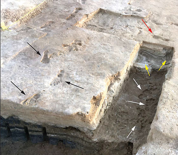
In 2002 a Polish geologist on holiday at the beach at Trachilos on Crete discovered a trackway on a bedding plane in shallow-marine Miocene sediments. It had been left by what seems to have been a bipedal hominin. Subsequent research was able to date the footprints to about 6.05 Ma. Though younger than Sahelanthropus, the discovery potentially challenges the exclusivity of hominins to Africa. Unsurprisingly, publication of this tentative interpretation drew negative responses from some quarters. But the discovery helped resurrect the notion that Africa may have been colonised in the Miocene by hominins that had evolved in Europe. That had been hinted at by the 1872 excavation of Oreopithecus bambolii from an Upper Miocene (~7.6 Ma) lignite mine in Tuscany, Italy – a year after publication of Darwin’s The Descent of Man.

Lignites in Tuscany and Sardinia have since yielded many more specimens, so the species is well documented. Oreopithecus could walk on two legs, its hands were capable of a precision grip and it had relatively small canines. Its Wikipedia entry cautiously refers to it as ‘hominid’ – i.e. lumped with all apes to comply with current taxonomic theory (above). In 2019 another fascinating find was made in a clay pit in Bavaria, Germany. Danuvius guggenmosi lived 11.6 Ma ago and fossilised remains of its leg- and arm bones suggested that it could walk on two legs: it too may have been on the hominin line. But no remains of Danuvius’s skull or teeth have been found. There is now an embarrassment of riches as regards Miocene fossil apes from Europe and the Eastern Mediterranean (Sevim-Erol, A. and 8 others 2023. A new ape from Türkiye and the radiation of late Miocene hominines. Nature Communications Biology, v. 6, article  842.; DOI: 10.1038/s42003-023-05210-5). A number of them closely resemble the earliest fossil hominins of Africa, but most predate the hominin record there by several million years.

Phylogenetic links between fossils assigned to Hominidae found in Africa and north of the Mediterranean Sea. (Credit: Sevim-Erol et al. 2023, Fig 5)

Ayla Sevim-Erol of Ankara University, Turkiye and colleagues from Turkiye, Canada and the Netherlands describe a newly identified Miocene genus, Anadoluvius, which they place in the Subfamily Homininae dated to around 8.7 Ma. Fragments of crania and partial male and female mandibles from Anatolia show that its canines were small and comparable with those of younger African hominins, such as Ardipithecus and Australopithecus. But limb bones are yet to be found. Around the size of a large male chimpanzee, Anadoluvius lived in an ecosystem remarkably like the grasslands and dry forests of modern East Africa, with early species of giraffes, wart hogs, rhinos, diverse antelopes, zebras, elephants, porcupines, hyenas and lion-like carnivores. Sevim-Erol et al. have attempted to trace back hominin evolution further than is possible with African fossils. They compare various skeletal features of different fossils and living genera to assess varying degrees of similarity between each genus, applied to 23 genera. These comprised 7 hominids from the African Miocene, 2 early African hominins (Ardipithecus and Orrorin) and 10 Miocene hominids from Europe and the Eastern Mediterranean. They also assessed similarities with 4 living genera, Homo, orang utan (Pongo), gorilla and chimp (Pan).

The resulting phylogeny shows close morphological links within a cluster (green ‘pools’ on diagram) of non-African hominids with the African hominins, gorillas, humans and chimps. There are less-close relations between that cluster and the earlier Miocene hominids of Africa (blue ‘pool’) and the possible phylogeny of orang utans (orange ‘pool’). Sevim-Erol et al. note that African hominins are clearly more similar and perhaps more closely related to the fossils of Europe and the Eastern Mediterranean than they are to Miocene African hominids. This suggests that evolution among the non-African hominids ceased around the end of the Miocene Epoch north of the Mediterranean Sea. But it may have continued in Africa. Somehow, therefore, it became possible late in Miocene times for hominids to migrate from Europe to Africa. Yet the earlier, phylogenetically isolated African hominids seem to have ‘crashed’ at roughly the same time. Such a complex scenario cannot be supported by phylogenetic studies alone: it needs some kind of ecological impetus.

The Mediterranean Basin at the end of the Miocene Epoch when the only water was in the deepest parts of the basin. (Credit: Wikipedia, Creative Commons)

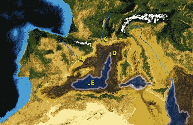
Following a ‘mild’ tectonic collision between the African continent and the Iberian Peninsula during the late Miocene connection between the Atlantic Ocean and the Mediterranean Sea was blocked from 6.0 to 5.3 Ma. Except for its deepest parts, seawater in the Mediterranean evaporated away to leave thick salt deposits. Rivers, such as the Rhône, Danube, Dneiper and Nile, shed sediments into the exposed basin. For 700 ka the basin was a fertile, sub-sea level plain, connecting Europe and North Africa over and E-W distance of 3860 km. There was little to stop the faunas of Eurasia and Africa migrating and intermingling, at a critical period in the evolution of the Family Hominidae. One genus presented with the opportunity was quite possibly the last common ancestor of all the hominins and chimps. The migratory window vanished at the end of the Miocene when what became the Strait of Gibraltar opened at 5.3 to allow Atlantic water. This resulted in the stupendous Zanclean flood with a flow rate about 1,000 times that of the present-day Amazon River. An animation of these events is worth watching

Earthquakes and flooding in the Ganges Basin

Floods pose a huge threat to the large populations of West Bengal, India and the state of Bangladesh, particularly in the highly fertile fluvio-deltaic plains of the Ganges and Brahmaputra. The two river systems drain 2 million km2 of the Eastern Himalaya of annual monsoon rains and snow melt, the first flowing west to east and the latter from east to west at the apex of the low-lying Bengal Basin. The 400 million people subsisting in the 105 thousand km2 onshore basin make it the world’s most populous delta plain with one of the highest population densities, averaging 1,100 per square kilometre in 2019. The risk of catastrophic flooding is generally ascribed to unusually high monsoonal precipitation and snow melt, combined with storm surges from the Bay of Bengal that funnels tropical cyclones. But either can bring inundation. Another factor has recently been proposed as an addition to flood hazard: earthquakes near the basin (Chamberlain, E.L and 12 others 2024. Cascading hazards of a major Bengal basin earthquake and abrupt avulsion of the Ganges River. Nature Communications, v. 15, online article 4975; DOI: 10.1038/s41467-024-47786-4). It seems they can completely and suddenly change the flow networks in such a complex system of major channels.

Using remotely sensed data Elizabeth Chamberlain, currently at Wageningen University in the Netherlands, and colleagues from Bangladesh, the US, Germany and Austria have detected an immense abandoned channel in the Ganges River. They reckon that it resulted from a sudden change in the river’s course. Such avulsions in the sluggish lower parts of a river system are generally caused by the flow becoming elevated above the flood plain by levees. When they burst free the channel may be abandoned. This one is 1.0 to 1.7 km wide and may have been the main Ganges channel at the time of avulsion. The main channel now flows about 45 km north of the abandoned relic. The event must have been sudden and irreversible as the relic channel contains a much thinner layer of fine mud deposited by stagnant water than in other abandoned channels that became ox-bow lakes. That implies rapid uplift and complete drainage from the channel. Throughout the Bengal Basin the immense high-water discharge and heavy sediment load seems generally to have infilled most abandoned channels, so this one is an anomaly.

Sand dykes along fractures in river alluvium of the Bengal Basin. (Credit: Chamberlain et al. Figs 3c and 3d)

Fieldwork near the old channel reveals fracturing of earlier riverbed sediments some of which are filled by intrusions of sand in the form of dykes up to 40 cm wide. Sand dykes are produced by liquefaction of sandy alluvium by seismic waves to slurry that can be injected into fractures pulled apart by seismic movements. The channel is now about 3 m below the level of the floodplain, suggesting subsidence since the avulsion event. Optically stimulated luminescence dating of sediment grains from the uppermost channel sands yielded ages averaging around 2.5 ka, marking the time when the sudden event took place. The authors consider that it marked a major reorganisation of the Ganges River system, involving catastrophic flooding. The nearest seismically active area is about 180 to 300 km to the east and northeast. Seismic modelling suggests that for liquefaction and fracturing to have affected the area of the abandoned channel the earthquake must have been of magnitude 7.5–8.0, possibly in the subduction zone that roughly follows the Bangladesh-Myanmar border. It may have had similar, yet to be demonstrated, effects throughout the eastern Bengal Basin.

There are no historic records of more recent massive earthquake-induced flooding of the Bengal Basin. However, global warming and growing human intervention in the Ganges-Brahmaputra river systems, such as large-scale dredging and industrialisation could make such events more likely. Other basins close to seismically active fault systems, such as the Yangtze and Yellow River basins of China, also face such risks.

Many thanks to  Piso Mojado for giving me the tip about this paper

Apology

Dear Followers

You will have noticed a 5-week break in my posting news items, for which I need to apologise and to explain.

Despite weekly searching all the leading journals that publish geoscientific papers, none have appeared that meet my criteria for commenting. That is, nothing has emerged that makes a significant breakthrough in any of the the Categories that Earth-logs covers. In fact, since Covid I have noticed a drop in the number of publications that do. Maybe there was a downturn in research during the pandemic, or perhaps some other reason such as a decline in the discipline, of journal policy changes.

There’s not much I can do other than wait patiently, and post when something turns up – you will be among the first to know about it, as ever!

In the meantime, maybe one or more of you have come across something interesting that I missed, or have a question about topics covered earlier. Either way, don’t hesitate to get in touch with me, either with a comment or using the Contact Author link in the Menu bar.

With regards

Steve Drury

The onset of weathering in the late Archaean and stabilisation of the continents

Distribution of exposed Archaean cratons. The blue Proterozoic areas may, in part be underlain by cratons. (Credit: Groves, D.I. & Santosh, M. DOI:10.1016/j.gr.2020.06.008)

About 50% of continental crust is of Archaean age (2.5 to 4.0 Ga) in huge blocks above lithosphere more than 150 km thick. Younger continental lithosphere is significantly thinner – as low as 40 km. Since the end of the Archaean Eon these blocks have remained tectonically stable and only show signs of extensional, brittle fracture that have been exploited by basaltic dyke swarms. Such crystalline monstrosities have remained rigid for 2.5 billion years. They are termed cratons from the Greek word κράτο (kratos) for ‘might’ or ‘strength’. Numbers of cratons have been pushed together by later tectonics to form continental ‘cores’, separated from one another by highly deformed ‘mobile belts’ formed by younger collisional orogenies. Africa and South America have 4 cratons each, Eurasia 6 or 7, the other continents all have one

Considering how much cratons have been stressed by later tectonic forces, their implacable rigidity might seem surprising. This rigidity is thought to be due to cratons’ unusually low amounts of the main heat-producing elements (HPE) potassium, uranium and thorium, the decay of whose radioactive isotopes produces surface heat flow. Cratons have the lowest surface heat flow on the planet, so in bulk they must have low HPE content. This stems from the nature of cratons’ deepest parts: almost anhydrous, once igneous rocks of intermediate average composition known as granulites. They formed by metamorphism of earlier crustal rocks at depths of up to 70km, which drove out most of their original HPEs and water. The upper cratonic crust has much the same complement of HPEs as that of more recent continental crust. This bulk depletion of cratons has maintained unusually low temperatures in their deep continental crust. That has been immune from partial melting and thus ductile deformation since it formed.

Three billion year-old TTG gneiss in the Outer Hebrides, Scotland. (Credit: British Geological Survey)

Jesse Reimink and Andrew Smye of Pennsylvania State University, USA have considered the geochemistry and history of the world’s cratons to address the long-standing issue of their stability and longevity (Reimink, J.R. & Smye, A.J. 2024. Subaerial weathering drove stabilization of continents. Nature, v. 629, online article; DOI: 10.1038/s41586-024-07307-1). Their main focus is on how the Archaean lower crust lost most of it HPEs, and where they went. During much of the Archaean continental crust formed by partial melting of hydrated basaltic rocks at shallow depths. That generated sodium-rich silicic magmas from which the dominant grey tonalite-trondhjemite-granodiorite (TTG) gneisses of Archaean crust formed by extreme ductile deformation. Though TTGs originally contained sufficient heat-producing capacity to make them ductile during the early Archaean there is little evidence that they underwent extensive partial melting themselves. But they did after 3.0 Ga to produce swarms of granite plutons in the upper Archaean crust.

Complementing the late-Archaean granite ‘swarm’ are deep-crustal granulites with low HPE contents, which mainly formed around the same time. The granulites contain highly metamorphosed sedimentary rocks, which seem to have been sliced into the Archaean crust during its ductile deformation phase. Some of them have compositions that suggest that they are derived from clay-rich shales, their proportion reaching about 30% of all granulite-facies metasediments. Clay minerals are the products of chemical weathering of silicon- and aluminium-rich igneous rocks exposed to the atmosphere. When they form, they host K, U and Th. Also, their composition and high initial water contents are conducive to partial melting under high-temperature conditions, to become a source of granitic magmas. Crustal weathering is key to Reimink and Smye’s hypothesis for the development of cratons in the late Archaean.

There is growing evidence that high Archaean heat flow through oceanic lithosphere – the mantle contained more undecayed HPE isotopes than now – reduced its density. As a result Archaean oceanic basins were considerably shallower than they became in later times. Because of the lower volume of the basins during the Archaean, seawater extended across much of the continental surface. For most of the Archaean Eon Earth was a ‘waterworld’, with little subaerial weathering of its TTG upper crust. As the volume of exposed continental crust increased so did surface weathering to form clay minerals that selectively absorbed HPEs. Over time shales became tectonically incorporated deep into the thickening Archaean continental crust to form a zone with increased heat producing capacity and a higher water content. Once deep enough and heated by their own content of HPE they began partially melting to yield voluminous granitic magmas to which they contributed their load of HPEs. Being lower in density than the bulk of TTG crust the granite melts would have risen to reach the upper crust. They also took in HPEs from the deep TTG crust itself. According to Reimink and Smye this would have concentrated continental heat production in the upper crust, leaving the deeper crust drier, less able to melt and assume ductile properties, and thus to create the cratons.

The authors believe that such a redistribution of heat production in the ancient continental crust did not need any major change in global tectonics. All it required was decreasing oceanic heat flow to create deeper and more voluminous ocean basins, allowing more continental surface to emerge above sea level and dynamic burial of sedimentary products of subaerial weathering. They conclude: “The geological record can then be cast in terms of a pre-emergence (TTG-dominated) and post-emergence (granite-dominated) planet.” That seems very neat … but it seems unlikely that samples can be drilled from the depths where the ‘action’ took place. Geologists depend on exposures of Archaean middle to deep crust brought to the surface by fortuitous later tectonics.

The chaotic early Solar System: when giant planets went berserk

Readers of Earth-logs will be familiar with the way gravitational interactions between the planets that orbit the Sun control cyclical shifts in each other’s rotational and orbital behaviours. The best known are the three Milankovich cycles. The eccentricity of Earth’s orbit (deviation from a circular path) changes according to the varying gravitational pulls exerted by Jupiter and Saturn as they orbit the Sun, and is dominated by 100 ka cyclicity. The tilt (obliquity) of Earth’s rotational axis changes in 41 ka cycles.  The direction in which the axis points relative to the Sun varies with its precession which has a period of about 25.7 ka. Together they control the amount of solar heating that our planet receives, best shown by the current variation in glacial-interglacial cycles. But the phenomena predicted by Milutin Milankovich show up in palaeoclimatic changes back to at least the late Precambrian. Climate changes resulting from the gravitational effect of Mars have recently been detected with a 2.4 Ma period. But that steady carousel of planetary motions hasn’t always characterised the Solar System.

Cartoon showing planet formation in the early, unstable Solar System (Credit: Mark Garlick, Science Source)

Observations of other stars that reveal the presence of their own planetary systems show that some have giant planets in much closer orbits than those that circuit the Sun. Others occur at distances that extend as far as the orbital diameters as those in the Solar System: so perhaps giant planets can migrate. A possibility began to be discussed in the late 1990s that Jupiter, Saturn, Uranus and Neptune – and a fifth now-vanished giant planet – were at the outset in neat, evenly-spaced and much closer orbits. But they were forced outwards later into more eccentric and generally askew orbits. In 2005, planetary astronomers gathered in Nice, France to ponder the possibilities. The outcome was the ‘Nice’ Model that suggested that a gravitational instability had once emerged, which set the Solar System in chaotic motion. It may even have flung gigantic masses, such as postulated fifth giant planets, into interstellar space. This upheaval may have been due to a rapid change in the overall distribution of mass in the Solar System, possibly involving gas and dust that had not yet accreted into other planets or their planetesimal precursors. Chaotic antics of monstrous bodies and shifts in their combined gravitational fields can barely be imagined: it was nothing like the staid and ever present Milankovich Effect. Geologists have reconstructed one gargantuan event that reset the chemistry of the early Earth when it collided with another body about the size of Mars. That  also flung off matter that became the Moon. Evidence from lunar and terrestrial zircon grains (see: Moon-forming impact dated; March 2009) suggests the collision occurred before 4.46 billion years ago (when parts of both eventually crystallised from magma oceans), Solar System having begun to form at around 4.57 Ga. Could formation of the Moon record the early planetary chaos? Others have suggested instead that the great upheaval was the Late Heavy Bombardment, between 4.1 and 3.8 Ga, which heavily cratered much of the lunar surface and those of moons orbiting the giant planets.

Another approach has been followed by Chrysa Avdellidou of the University of Leicester, UK and colleagues from France and the US (Avdellidoli, C. et al. 2024. Dating the Solar System’s giant planet orbital instability using enstatite meteorites. Science, v. 384, p. 348-352; DOI: 10.1126/science.adg8092) after discovery of a new family of asteroids: named after its largest member Athor. The composition of their surfaces, from telescopic spectra, closely matches that of EL enstatite chondrite meteorites. Dating these meteorites should show when their parent asteroids – presumably the Athors – formed.  Using argon and xenon isotopes Mario Trieloff  and colleagues from the University of Heidelberg, Germany in showed that the materials in EL enstatite chondrite meteorites were assembled a mere 2 Ma after the Solar System formed (Trieloff, M. et al. 2022. Evolution of the parent body of enstatite (EL) chondrites. Icarus, v. 373, article 114762; DOI: 10.1016/j.icarus.2021.114762). Be that as it may, that the evidence came from small meteorites shows that the parent body, estimated as having had a 240 to 420 km diameter, was shattered at some later time. Moreover, at that very early date such bodies would have contained a ready heat source in the form of a short-lived isotope of aluminium (26Al) which decays to stable 26Mg, with a half-life of 0.717 Ma. 26Al is thought to have been produced by a supernova that has been suggested to have triggered the formation of the Solar System. Excessive 26Mg is found in many meteorites, evidence for metamorphism formed by such radiogenic heat. They also record the history of their cooling.

Avdellidoli et al. estimate that the 240 to 420 km Athor parental planetesimal had slowly cooled for at least 60 Ma after it formed. When it was shattered, the small fragments would have cooled instantaneously to the temperature of interplanetary space – a few degrees above absolute zero (-273.2 °C). From this they deduce the age of the chaotic restructuring of the early Solar System to be at least 60 Ma after its formation. Other authors use similar reasoning from other chondritic meteorite classes to suggest it may have happened even earlier at 11 Ma. But there are other views for a considerably later migration of the giant planets and the havoc that they wrought. The only widely agreed date, in what seems to be an outbreak of wrangling among astronomers, is for the Moon-forming collision: 110 Ma after formation of the Solar System. For me, at least, that’s good-enough evidence for when system-wide chaos prevailed. The Late Heavy Bombardment between 4.1 and 3.8 Ga seems to require a different mechanism as it affected large bodies that still exist. It may have resulted from whatever formed the asteroid belt, for it was bodies within the range of sizes of the asteroids that did the damage, in both the Inner and Outer Solar System.

See also: The instability at the beginning of the solar system. MSUToday, 27 April 2022: Voosen, P. 2024. Giant planets ran amok soon after the Solar System’s birth. Science, v. 384 news article eadp8889; DOI: 10.1126/science.adp8889

The peptide bond that holds life together may have an interstellar origin

In the 1950s Harold Urey of the University of Chicago and his student Stanley Miller used basic lab glassware containing 200 ml of water and a mix of the gases methane (CH4), ammonia (NH3) and hydrogen sulfide (H2S) to model conditions on the early Earth. Heating this crude analogue for ocean and atmosphere and continuous electrical discharge through it did, in a Frankensteinian manner, generate amino acids. Repeats of the Miller-Urey experiment have yielded 10 of the 20 amino acids from which the vast array of life’s proteins have been built. Experiments along similar lines have also produced the possible precursors of cell walls – amphiphiles. In fact, all kinds of ‘building blocks’ for life’s chemistry turn up in analyses of carbonaceous chondrite meteorites and in light spectra from interstellar gas clouds. The ‘embarrassment of riches’ of life’s precursors from what was until the 20th century regarded as the ‘void’ of outer space lacks one thing that could make it a candidate for life’s origin, or at least for precursors of proteins and the genetic code DNA and RNA. Both kinds of keystone chemicals depend on a single kind of connector in organic chemistry.

Reaction between two molecules of the amino acid glycene that links them by a peptide bond to form a dipeptide. (Credit: Wikimedia Commons)

Molecules of amino acids have acidic properties (COOH – carboxyl) at one end and their other end is basic (NH2 – amine). Two can react by their acid and basic ‘ends’ neutralising. A hydroxyl (OH) from carboxyl and a proton (H+) from amine produce water. This gives the chance for an end-to-end linkage between the nitrogen and carbon atoms of two amino acids – the peptide bond. The end-product is a dipeptide molecule, which also has carboxyl at one end and amine at the other. This enables further linkages through peptide bonds to build chains or polymers based on amino acids – proteins. Only 20 amino acids contribute to terrestrial life forms, but linked in chains they can form potentially an unimaginable diversity of proteins. Formation of even a small protein that links together 100 amino acids taken from that small number illustrates the awesome potential of the peptide bond. The number of possible permutations and combinations to build such a protein is 20100 – more than the estimated number of atoms in the observable universe! Protein-based life has almost infinite options: no wonder that ecosystems on Earth are so diverse, despite using a mere 20 building blocks. Simple amino acids can be chemically synthesised from C, H, O and N. About 500 occur naturally, including 92 found in a single carbonaceous chondrite meteorite. They vastly increase the numbers of conceivable proteins and other chain-molecules analogous to RNA and DNA: a point seemingly lost on exobiologists and science fiction writers!

Serge Kranokutski of the Max Planck Institute for Astronomy at the Friedrich Schiller University in Jena, German and colleagues from Germany, the Netherlands and France have assessed the likelihood of peptides forming in interstellar space in two publications (Kranokutski S.A. and 4 others 2022. A pathway to peptides in space through the condensation of atomic carbon. Nature Astronomy, v, 6, p. 381–386; DOI: 10.1038/s41550-021-01577-9. Kranokutski, S.A. et al. 2024. Formation of extraterrestrial peptides and their derivatives. Science Advances, v. 10, article eadj7179; DOI: 10.1126/sciadv.adj7179). In the first paper the authors show experimentally that condensation of carbon atoms on cold cosmic dust particles can combine with carbon monoxide (CO) and ammonia (NH3) form amino acids. In turn, they can polymerise to produce peptides of different lengths. The second demonstrates that water molecules, produced by peptide formation, do not prevent such reactions from happening. In other words, proteins can form inorganically anywhere in the cosmos. Delivery of these products, through comets or meteorites, to planets forming in the habitable ‘Goldilocks’ zone around stars may have been ‘an important element in the origins of life’ – anywhere in the universe. Chances are that, compared with the biochemistry of Earth, such life would be alien in an absolute sense. There are effectively infinite options for the proteins and genetic molecules that may be the basis of life elsewhere, quite possibly on Mars or the moons of Jupiter and Saturn: should it or its chemical fossils be detectable.

The first Europeans at the Ukraine-Hungary border

Until this year, the earliest date recorded for the presence of humans in Europe came from the Sierra de Atapuerca in the Province of Burgos, northern Spain. The Sima del Elefante cave yielded a fossil mandible of a human dubbed Homo antecessor from which an age between 1.2 to 1.1 Ma was estimated from a combination of palaeomagnetism, cosmogenic nuclides and stratigraphy. Stone tools from the Vallonet Cave in southern France are around the same age. There is a time gap of about 200 ka before the next sign of human ventures into Europe, probably coinciding with an extreme ice age. They reappear in the form of stone tools and even footprints that they left between 1.0 to 0.78 Ma in ancient river sediments beneath the crumbling sea cliffs of Happisburgh in Norfolk, England. Although no human fossils were preserved, they too have been assigned to H. antecessor.

Topographic map of Europe (click to see full resolution in a new window). The Carpathian Mountains form an arc surrounding the Pannonian Basin (Hungarian Plains) just below centr. Korolevo and other Homo erectus and H. antecessor sites are marked by red spots (Credit: Wikipedia Commons)

In 1974 Soviet archaeologists discovered a site bearing stone tools by the River Tisza at Korolevo in the Carpathian Mountains close to the borders between Ukraine, Romania and Hungary. Korolevo lies at the northeastern edge of the Pannonian Basin that dominates modern Hungary. Whoever left the tools was on the westward route to a huge, fertile area whose game might support them and their descendants. The route along the Tisza leads to the River Danube and then to its headwaters far to the west. Going eastwards leads to the plains north of the Black Sea and eventually via Georgia to the Levant. On that route lies Dmanisi in Georgia, famous for the site where remains of the first hominins (H. erectus, dated at ~1.8 Ma) to leave Africa were found (see: Consider Homo erectus for what early humans achived). The tools from Korolevo are primitive, but have remained undated since 1974. 50 years on, Roman Garba of the Czech Academy of Sciences with colleagues from Czechia, Ukraine, Germany, Australia, South Africa and Denmark have finally resolved their antiquity (Garba, R. and 12 others 2024. East-to-west human dispersal into Europe 1.4 million years ago. Nature v. 627, p. 805–810; DOI: 10.1038/s41586-024-07151-3). Without fossils it is not possible to decide if the tool makers were H. erectus or H. antecessor.

The method used to date the site is based on radioactive 10Be and 26Al formed from oxygen and silicon in quartz grains by cosmic ray bombardment while the grains are at the surface. Since the half life of 26Al (0.7 Ma) is less than that of 10Be (1.4 Ma), after burial the 26Al/10Be ratio decreases and is a guide to the age of the sediment layer that contains the quartz grains. In this case the ag is quite precise (1.42 ± 0.28 Ma). The decreasing age of H. erectus or H. antecessor sites from the 1.8 Ma of Dmanisi in Georgia in the east, through 1.4 Ma (Korolevo) to 1.2 in Spain and France could mark the slow westward migration of the earliest Europeans. It is tempting to suggest possible routes as Garba et al. have. But such sparse and widely separated sites can yield very little certainty. Indeed, it is equally likely that each known site marks the destination of separate migrations at different times that ended in population collapse. The authors make an interesting point regarding the Korolevo population. They were there at a time when three successive interglacials were significantly warmer than the majority during the Early Pleistocene. Also glacial cycles then had ~41 ka time spans before the transition to 100 ka about 1 Ma ago. Unfortunately, no information about the ecosystem that the migrants exploited is available

See also: Prostak, S. 2024. 1.4-Million-Year-Old Stone Tools Found in Ukraine Document Earliest Hominin Occupation of Europe. Sci News, 7 March 2024. (includes map showing possible routes of early human dispersal)

Ocean-floor sediments reveal the influence of Mars on long-term climate cycles

In 1976 three scientists from Columbia and Brown (USA) and Cambridge (UK) Universities published a paper that revolutionised the study of ancient climates (Hays J.D., Imbrie J. and Shackleton N.J. 1976. Variations in the Earth’s Orbit: Pacemaker of the Ice Ages. Science, v. 194, p. 1121-1132;  DOI: 10.1126/science.194.4270.1121). Using variations in oxygen isotopes from foraminifera through two cores of sediments beneath the floor of the southern Indian Ocean they verified Milutin Milankovich’s hypothesis of astronomical controls over Earth’s climate. This centred on changes in Earth’s orbital parameters induced by gravitational effects from the motions of other planets: its orbit’s eccentricity, and the tilt and precession of its rotational axis. Analysis of the frequency of isotopic variations in the resulting time series yielded Milankovich’s predictions of ~100, 41 and 21 ka periodicities respectively. The time spanned by the cores was that of the last 500 ka of the Pleistocene and thus the last 5 glacial-interglacial cycles. Subsequently, the same astronomical climate forcing  has been detected  for various climate-induced changes in the earlier sedimentary record, including the glacial cycles of the Carboniferous and Neoproterozoic, Jurassic climate changes due to oceanic methane emissions and many other types of cyclicity during the Phanerozoic.

One hemisphere of Mars captured by ESA’s Mars Express. Credit: ESA / DLR / FU Berlin /

As well as time series based on isotopic and other geochemical changes in marine cores, other variables such as thickness of turbidite beds or cyclical repetitions of short rock sequences such as the ‘cyclothems’ of Carboniferous age (repetitions of a  limestone, sandstone, soil, coal sequence) have also been subject to frequency analysis. Sedimentary features that have not been tried are gaps or hiatuses in stratigraphic sequences where strata are missing from a deep-sea sequence. These signify erosion of sediment due to vigorous bottom currents in sequences otherwise dominated by continuous deposition under low-energy conditions. Three geoscientists from the University of Sydney, Australia and the Sorbonne University, France, have subjected records of gaps in Cenozoic sedimentation from 293 deep-sea drill cores to time-series analysis to discover what such ‘big data’ might reveal as regards climate fluctuations on the order of millions of years (Dutkiewicz, A., Boulila, S. & Müller, R.D. 2024. Deep-sea hiatus record reveals orbital pacing by 2.4 Myr eccentricity grand cycles. Nature Communications, v. 15, article 1998; DOI: 10.1038/s41467-024-46171-5).

In theory gravitational interrelationships between all the orbiting planets should have an effect on the orbital parameters of each other, and thus the amount of received solar radiation and changes in global climate. As well as the Milankovich effect, longer astronomical ‘grand cycles’ may therefore have been reflected somehow in Earth’s climatic history (Laskar, J. et al. 2004. A long-term numerical solution for the insolation quantities of the Earth. Astronomy & Astrophysics, v. 428, p. 261-285; DOI: 10.1051/0004-6361:20041335). Based on Laskar et al.’s calculations Adriana Dutkiewicz and colleagues sought evidence for two predicted ‘grand cycles’ that result from orbital interactions between Earth and Mars. These are a 2.4 Ma period in the eccentricity of Earth’s orbit and one of 1.2 Ma in the tilt of its axis.

The authors were able to detect cyclicity in the hiatus time series that is close to the 2.4 Ma Mars-induced waxing and waning of solar heating. Warming would increase mixing of ocean water through cyclones and hurricanes. That would then induce more energetic deep ocean currents and more erosion on the deep ocean floor: more gaps in sedimentation. Cooler conditions would ‘calm’ deep ocean currents so that deposition would outweigh evidence of erosion. The 1.2 Ma axial tilt cyclicity is not apparent in the data. Interestingly, the ~2.4 Ma cyclicity underwent a significant deviation at the Palaeocene-Eocene Boundary’ (56Ma), seemingly predicted by Laskar et al’s  astronomical solutions as a chaotic orbital transition between 56 and 53 Ma. Dutkiewicz et al. also chart the relations between the sedimentary-hiatus time series and major tectonic, oceanographic, and climatic changes during the Cenozoic Era, and found that terrestrial processes did disrupt the Mars-related orbital eccentricity cycles.

The findings suggest that long-term astronomical climate forcing needs to be borne in mind for better understanding the future response of the ocean to global warming. Also, if Mars had such an influence so must have Venus, which is more massive and closer. That remains to be investigated, and also the effects of the giant planets. In the very distant past there behaviour may have resulted in unimaginable astronomical changes. According to the bizarrely named Nice Model a back and forth shuffling of the Giant Planets was probably responsible for the Late Heavy Bombardment 4.1 to 3.8 billion years (Ga) ago. Such errant behaviour may even have triggered the flinging of some of the Sun’s original planetary complement out of the solar system and changed the outward order of the existing eight. Fortunately, the present planetary set-up seems to be stable …

See also: Dutkiewicz, A., & Müller, R. D. 2022. Deep-sea hiatuses track the vigor of Cenozoic ocean bottom currents. Geology, v. 50, p. 710–715; DOI: 10.1130/G49810.1; Mars drives deep-ocean circulation in Earth’s oceans, study suggests. Sci News, 13 March 2024.

How did African humans survive the 74 ka Toba volcanic supereruption?

The largest volcanic eruption during the 2.5 million year evolution of the genius Homo, about 74 thousand years (ka) ago, formed a huge caldera in Sumatra, now filled by Lake Toba. A series of explosions lasting just 9 to 14 days was forceful enough to blast between 2,800 to 6,000 km3 of rocky debris from the crust. An estimated 800 km3 was in the form of fine volcanic ash that blanketed South Asia to a depth of 15 cm. Thin ash layers containing shards of glass from Toba occur in marine sediments beneath the Indian Ocean, the Arabian and South China Seas. Some occur as far off as sediments on the floor of Lake Malawi in southern Africa. A ‘spike’ of sulfates is present at around 74 ka in a Greenland ice core too. Stratospheric fine dust and sulfate aerosols from Toba probably caused global cooling of up to 3.5 °C over a modelled 5 years following the eruption. To make matters worse, this severe ‘volcanic winter’ occurred during a climatic transition from warm to cold caused by changes in ocean circulation and falling atmospheric CO2 concentration, known as a Dansgaard-Oeschger event.

There had been short-lived migrations of modern humans out of Africa into the Levant since about 185 ka. However, studies of the mitochondrial DNA (mtDNA) of living humans in Eurasia and Australasia suggest that permanent migration began about 60 ka ago. Another outcome of the mtDNA analysis is that the genetic diversity of living humans is surprisingly low. This suggests that human genetic diversity may have been sharply reduced globally roughly around the time of the  Toba eruption. This implies a population bottleneck with the number of humans alive at the time to the order of a few tens of thousands (see also: Toba ash and calibrating the Pleistocene record; December 2012). Could such a major genetic ‘pruning’ have happened in Africa? Over six field seasons, a large team of geoscientists and archaeologists drawn from the USA, Ethiopia, China, France and South Africa have excavated a rich Palaeolithic site in the valley of the Shinfa River, a tributary of the Blue Nile in western Ethiopia. Microscopic studies of the sediments enclosing the site yielded glass shards whose chemistry closely matches those in Toba ash, thereby providing an extremely precise date for the human occupation of the site: during the Toba eruption itself (Kappelman, Y. and 63 others 2024. Adaptive foraging behaviours in the Horn of Africa during Toba supereruption. Nature, v. 627; DOI: 10.1038/s41586-024-07208-3).

Selection of possible arrowheads from the Shinfa River site (Credit: Kappelman et al.; Blue Nile Survey Project)

The artifacts and bones of what these modern humans ate suggest a remarkable scenario for how they lived. Stone tools are finely worked from local basalt lava, quartz and flint-like chalcedony found in cavities in lava flows. Many of them are small, sharp triangular points, some of which show features consistent with their use as projectile tips that fractured on impact; they may be arrowheads, indeed the earliest known. Bones found at the site are key pointers to their diet. They are from a wide variety of animal, roughly similar to those living in the area at present: from monkeys to giraffe, guinea fowl to ostrich, and even frogs. There are remains of many fish and freshwater molluscs. Although there are no traces of plant foods, clearly those people who loved through the distant effects of Toba were well fed. Although a period of global cooling may have increased aridity at tropical latitudes in Africa, the campers were able to devise efficient strategies to obtain victuals. During wet seasons they lived off terrestrial prey animals, and during the driest times ate fish from pools in the river valley. These are hardly conditions likely to devastate their numbers, and the people seem to have been technologically flexible. Similar observations were made at the Pinnacle Point site in far-off South Africa in 2018, where Toba ash is also present. Both sites refute any retardation of human cultural progress 74 ka ago. Rather the opposite: people may have been spurred to innovation, and the new strategies may have allowed them to migrate more efficiently, perhaps along seasonal drainages. In this case that would have led them or their descendants to the Nile and a direct route to Eurasia; along ‘blue highway’ corridors as Kappelman et al. suggest.

Yet the population bottleneck implied by mtDNA analyses is only vaguely dated: it may have been well before or well after Toba. Moreover, there is a 10 ka gap between Toba and the earliest accurately dated migrants who left Africa – the first Australians at about 65 ka. However, note that there is inconclusive evidence that modern humans may have occupied Sumatra by the time of the eruption.  Much closer to the site of the eruption in southeast India, stone artifacts have been found below and above the 74 ka datum marked by the thick Toba Ash. Whether these were discarded by anatomically modern humans or earlier migrants such as Homo erectus remains unresolved. Either way, at that site there is no evidence for any mass die-off, even though conditions must have been pretty dreadful while the ash fell. But that probably only lasted for little more than a month. If the migrants did suffer very high losses to decrease the genetic diversity of the survivors, it seems just as likely to have been due to attrition on an extremely lengthy trek, with little likelihood of tangible evidence surviving. Alternatively, the out-of-Africa migrants may have been small in number and not fully representative of the genetic richness of the Africans who stayed put: a few tens of thousand migrants may not have been very diverse from the outset.

The ‘Anthropocene Epoch’ bites the dust?

The International Commission on Stratigraphy (ICS) issues guidance for the division of geological history that has evolved from the science’s original approach: that was based solely on what could be seen in the field. That included: variations in lithology and the law of superposition; unconformities that mark interruptions through deformation, erosion and renewed deposition; the fossil content of sediments and the law of faunal succession; and more modern means of division, such as geomagnetic changes detected in rock over time. That ‘traditional’ approach to relative time is now termed chronostratigraphy, which has evolved since the 19th century from the local to the global scale as geological research widened its approach. Subsequent development of various kinds of dating has made it possible to suggest the actual, absolute time in the past when various stratigraphic boundaries formed – geochronology. Understandably, both are limited by the incompleteness of the geological record – and the whims of individual geologists. For decades the ICS has been developing a combination of both approaches that directly correlates stratigraphic units and boundaries with accurate geochronological ages. This is revised periodically, the ICS having a detailed protocol for making changes.  You can view the Cenozoic section of the latest version of the International Chronostratigraphic Chart and the two systems of units below. If you are prepared to travel to a lot of very remote places you can see a monument – in some cases an actual Golden Spike – marking the agreed stratigraphic boundary at the ICS-designated type section for 80 of the 93 lower boundaries of every Stage/Age in the Phanerozoic Eon. Each is a sonorously named Global Boundary Stratotype Section and Point or GSSP (see: The Time Lords of Geology, April 2013). There are delegates to various subcommissions and working groups of the ICS from every continent, they are very busy and subject to a mass of regulations

Chronostratigraphic Chart for the Cenozoic Era showing the 5 tiers of stratigraphic time division. The little golden spikes mark where a Global Boundary Stratotype Section and Point monument has been erected at the boundary’s type section.

On 11 May 2011, the Geological Society of London hosted a conference, co-sponsored by the British Geological Survey, to discuss evidence for the dawn of a new geological Epoch: the Anthropocene, supposedly marking the impact of humans on Earth processes. There has been ‘lively debate’ about whether or not such a designation should be adopted. An Epoch is at the 4th tier of the chronostratigraphic/geochronologic systems of division, such as the Holocene, Pleistocene, Pliocene and Miocene, let alone a whole host of such entities throughout the Phanerozoic, all of which represent many orders of magnitude longer spans of time and a vast range of geological events. No currently agreed Epoch lasted less than 11.7 thousand years (the Holocene) and all the others spanned 1 Ma to tens of Ma (averaged at 14.2 Ma). Indeed, even geological Ages (the 5th tier) span a range from hundreds of thousands to millions of years (averaged at 6 Ma). Use ‘Anthropocene’ in Search Earth-logs to read posts that I have written on this proposal since 2011, which outline the various arguments for and against it.

In the third week of May 2019 the 34-member Anthropocene Working Group (AWG) of the ICS convened to decide on when the Anthropocene actually started. The year 1952 was proposed – the date when long-lived radioactive plutonium first appears in sediments before the 1962 International Nuclear Test-Ban Treaty. Incidentally, the AWG proposed a GSSP for the base of the Anthropocene in a sediment core through sediments in the bed of Crawford Lake an hour’s drive west of Toronto, Canada.   After 1952 there are also clear signs that plastics, aluminium, artificial fertilisers, concrete and lead from petrol began to increase in sediments. The AWG accepted this start date (the Anthropocene ‘golden spike’) by a 29 to 5 vote, and passed it into the vertical ICS chain of decision making. This procedure reached a climax on Monday 4 March 2024, at a meeting of the international Subcommission on Quaternary Stratigraphy (SQS): part of the ICS. After a month-long voting period, the SQS announced a 12 to 4 decision to reject the proposal to formally declare the Anthropocene as a new Epoch. Normally, there can be no appeals for a losing vote taken at this level, although a similar proposal may be resubmitted for consideration after a 10 year ‘cooling off’ period. Despite the decisive vote, however, the chair of the SQS, palaeontologist Jan Zalasiewicz of the University of Leicester, UK, and one of the group’s vice-chairs, stratigrapher Martin Head of Brock University, Canada have called for it to be annulled, alleging procedural irregularities with the lengthy voting procedure.

Had the vote gone the other way, it would marked the end of the Holocene, the Epoch when humans moved from foraging to the spread of agriculture, then the ages of metals and ultimately civilisation and written history. Even the Quaternary Period seemed under threat: the 2.5 Ma through which the genus Homo emerged from the hominin line and evolvd. Yet a pro-Anthropocene vote would have faced two more, perhaps even more difficult hurdles: a ratification vote by the full ICS, and a final one in August 2024 at a forum of the International Union of Geological Sciences (IUGS), the overarching body that represents all aspects of geology.  

There can be little doubt that the variety and growth of human interferences in the natural world since the Industrial Revolution poses frightening threats to civilisation and economy. But what they constitute is really a cultural or anthropological issue, rather than one suited to geological debate. The term Anthropocene has become a matter of propaganda for all manner of environmental groups, with which I personally have no problem. My guess is that there will be a compromise. There seems no harm either way in designating the Anthropocene informally as a geological Event. It would be in suitably awesome company with the Permian and Cretaceous mass extinctions, the Great Oxygenation Event at the start of the Proterozoic, the Snowball Earth events and the Palaeocene–Eocene Thermal Maximum. And it would require neither special pleading nor annoying the majority of geologists. But I believe it needs another name. The assault on the outer Earth has not been inflicted by the vast majority of humans, but by a tiny minority who wield power for profit and relentless growth in production. The ‘Plutocracene’ might be more fitting. Other suggestions are welcome …

See also: Witze, A. 2024. Geologists reject the Anthropocene as Earth’s new epoch — after 15 years of debate. Nature, v. 627, News article; DOI: 10.1038/d41586-024-00675-8; Voosen, P. 2024. The Anthropocene is dead. Long live the Anthropocene. Science, v. 383, News article, 5 March 2024.

A new explanation for the Neoproterozoic Snowball Earth episodes

The Cryogenian Period that lasted from 860 to 635 million years ago is aptly named, for it encompassed two maybe three episodes of glaciation. Each left a mark on every modern continent and extended from the poles to the Equator. In some way, this series of long, frigid catastrophes seems to have been instrumental in a decisive change in Earth’s biology that emerged as fossils during the following Ediacaran Period (635 to 541 Ma). That saw the sudden appearance of multicelled organisms whose macrofossil remains – enigmatic bag-like, quilted and ribbed animals – are found in sedimentary rocks in Australia, eastern Canada and NW Europe. Their type locality is in the Ediacara Hills of South Australia, and there can be little doubt that they were the ultimate ancestors of all succeeding animal phyla. Indeed one of them Helminthoidichnites, a stubby worm-like animal, is a candidate for the first bilaterian animal and thus our own ultimate ancestor. Using the index for Palaeobiology or the Search Earth-logs pane you can discover more about them in 12 posts from 2006 to 2023. The issue here concerns the question: Why did Snowball Earth conditions develop? Again, refresh your knowledge of them, if you wish, using the index for Palaeoclimatology or Search Earth-logs. From 2000 onwards you will find 18 posts: the most for any specific topic covered by Earth-logs. The most recent are Kicking-off planetary Snowball conditions (August 2020) and Signs of Milankovich Effect during Snowball Earth episodes (July 2021): see also: Chapter 17 in Stepping Stones.

One reason why Snowball Earths are so enigmatic is that CO2 concentrations in the Neoproterozoic atmospheric were far higher than they are at present. In fact since the Hadean Earth has largely been prevented from being perpetually frozen over by a powerful atmospheric greenhouse effect. Four Ga ago solar heating was about 70 % less intense than today, because of the ‘Faint Young Sun’ paradox. There was a long episode of glaciation (from 2.5 to 2.2 Ga) at the start of the Palaeoproterozoic Era during which the Great Oxygenation Event (GOE) occurred once photosynthesis by oxygenic bacteria became far more common than those that produced methane. This resulted in wholesale oxidation to carbon dioxide of atmospheric methane whose loss drove down the early greenhouse effect – perhaps a narrow escape from the fate of Venus. There followed the ‘boring billion years’ of the Mesoproterozoic during which tectonic processes seem to have been less active. in that geologically tedious episode important proxies (carbon and sulfur isotopes) that relate to the surface part of the Earth System ‘flat-lined’.  The plethora of research centred on the Cryogenian glacial events seems to have stemmed from the by-then greater complexity of the Precambrian Earth System.

Since the GOE the main drivers of Earth’s climate have been the emission of CO2 and SO2 by volcanism, the sedimentary burial of carbonates and organic carbon in the deep oceans, and weathering. Volcanism in the context of climate is a two-edged sword: CO2 emission results in greenhouse warming, and SO2 that enters the stratosphere helps reflect solar radiation away leading to cooling. Silicate minerals in rocks are attacked by hydrogen ions (H+) produced by the solution of CO2 in rain water to form a weak acid (H2CO3: carbonic acid). A very simple example of such chemical weathering is the breakdown of calcium silicate:

CaSiO3  +  2CO2  + 3H2O  =  Ca2+  +  2HCO3  +  H4SiO4  

The reaction results in calcium and bicarbonate ions being dissolved in water, eventually to enter the oceans where they are recombined in the shells of planktonic organisms as calcium carbonate. On death, their shells sink and end up in ocean-floor sediments along with unoxidised organic carbon compounds. The net result of this part of the carbon cycle is reduction in atmospheric CO2 and a decreased greenhouse effect: increased silicate weathering cools down the climate. Overall, internal processes – particularly volcanism – and surface processes – weathering and carbonate burial – interact. During the ‘boring billion’ they seem to have been in balance. The two processes lie at the core of attempts to model global climate behaviour in the past, along with what is known about developments in plate tectonics – continental break-up, seafloor spreading and orogenies – and large igneous events resulting from mantle plumes. A group of geoscientists from the Universities of Sydney and Adelaide, Australia have evaluated the tectonic factors that may have contributed to the first and longest Snowball Earth of the Neoproterozoic: the Sturtian glaciation (717 to 661 Ma) (Dutkiewicz, A. et al. 2024. Duration of Sturtian “Snowball Earth” glaciation linked to exceptionally low mid-ocean ridge outgassing. Geology, v. 52, online early publication; DOI: 10.1130/G51669.1).

Palaeogeographic reconstructions (Robinson projection) during the early part of the Sturtian global glaciation: LEFT based on geological data from Neoproterozoic terrains on modern continents; RIGHT based on palaeomagnetic pole positions from those terrains. Acronyms refer to each terrains, e.g. Am is Amazonia, WAC is the West African Craton. Orange lines are ocean ridges, those with teeth are subduction zone. (Credit: Dutkiewicz et al., parts of Fig. 1)

Shortly before the Sturtian began there was a major flood volcanism event, forming the Franklin large igneous province, remains of which are in Arctic Canada. The Franklin LIP is a subject of interest for triggering the Sturtian, by way of a ‘volcanic winter’ effect from SO2 emissions or as a sink for CO through its weathering. But both can be ruled out as no subsequent LIP is associated with global cooling and the later, equally intense Marinoan global glaciation (655 to 632 Ma) was bereft of a preceding LIP. Moreover, a world of growing frigidity probably could not sustain the degree of chemical weathering to launch a massive depletion in atmospheric CO2. In search of an alternative, Adriana Dutkiewicz and colleagues turned to the plate movements of the early Neoproterozoic. Since 2020 there have been two notable developments in modelling global tectonics of that time, which was dominated by the evolution of the Rodinia supercontinent. One is based largely on geological data from the surviving remnants of Rodinia (download animation), the other uses palaeomagnetic pole positions to fix their relative positions: the results are very different (download animation).

Variations in ocean ridge lengths, spreading rates and oceanic crust production during the Neoproterozoic estimated from the geological (orange) and palaeomagnetic (blue) models. Credit: Dutkiewicz et al., parts of Fig. 2)

The geology-based model has Rodinia beginning to break up around 800 Ma ago with a lengthening of global constructive plate margins during disassembly. The resulting continental drift involved an increase in the rate of oceanic crust formation from 3.5 to 5.0 km2 yr-1. Around 760 Ma new crust production more than halved and continued at a much slowed rate throughout the Cryogenian and the early part of the Ediacaran Period.  The palaeomagnetic model delays breakup of the Rodinia supercontinent until 750 Ma, and instead of the rate of crust production declining through the Cryogenian it more than doubles and remains higher than in the geological model until the late Ediacaran. The production of new oceanic crust is likely to govern the rate at which CO2 is out-gassed from the mantle to the atmosphere. The geology-based model suggests that from 750 to 580 Ma annual CO2 additions could have been significantly below what occurred during the Pleistocene ice ages since 2.5 Ma ago. Taking into account the lower solar heat emission, such a drop is a plausible explanation for the recurrent Snowball Earths of the Neoproterozoic. On the other hand, the model based on palaeomagnetic data suggests significant warming during the Cryogenian contrary to a mass of geological evidence for the opposite.

A prolonged decrease in tectonic activity thus seems to be a plausible trigger for global glaciation. Moreover, reconstruction of Precambrian global tectonics using available palaeomagnetic data seems to be flawed, perhaps fatally. One may ask, given the trends in tectonic data: How did the Earth repeatedly emerge from Snowball episodes? The authors suggest that the slowing or shut-down of silicate weathering during glaciations allowed atmospheric CO2 to gradually build up as a result of on-land volcanism associated with subduction zones that are a quintessential part of any tectonic scenario.

This kind of explanation for recovery of a planet and its biosphere locked in glaciation is in fact not new. From the outset of the Snowball Earth hypothesis much the same escape mechanisms were speculated and endlessly discussed. Adriana Dutkiewicz and colleagues have fleshed out such ideas quite nicely, stressing a central role for tectonics. But the glaring disparities between the two models show that geoscientists remain ‘not quite there’. For one thing, carbon isotope data from the Cryogenian and Ediacaran Periods went haywire: living processes almost certainly played a major role in the Neoproterozoic climatic dialectic.

Neanderthals and the earliest ‘plastic’ handles

February 2024 was a notable month for discoveries about ancient technology: first that of an ancient tool probably used in rope making and now signs of the use of a composite ‘plastic’ material in stone-tool hafts. Both are from Neanderthal sites in France, the first dated around 52 to 41 ka and the second in the Le Moustier rock shelters of the Dordogne – the type locality for the Mousterian culture associated with Neanderthals (Schmidt, P. et al. 2024. Ochre-based compound adhesives at the Mousterian type-site document complex cognition and high investment. Science Advances, v. 10, article ead10822; DOI: 10.1126/sciadv.adl0822), dated at around 56 to 40 ka. The second discovery resulted from the first detailed analysis of unstudied artifacts unearthed from Le Moustier in 1907 by Swiss archaeologist Otto Hauser that had been tucked away in a Berlin Museum.

Patrick Schmidt of the University of Tubingen in Germany and colleagues  from Germany, the US and Kazakhstan identified stone artifacts that show traces of red and yellow colorants. At first sight it could be suggested that they are decorations of some kind. However, they coat only parts of the stone flakes and are sharply distinct from the fresh rock surface and the sharpest edges. Another feature discovered during chemical analysis is that the colour is due to iron hydroxides (goethite) but this ochre is mixed with natural bitumen: the coating is a composite of an adhesive and filler not far different from what can be purchased in any hardware store.

LEFT: Stone flake from the Le Moustier site in France, partly coated with a reddish iron-rich colorant. RIGHT: Experimental stone flakes with 55:44 mix of goethite and bitumen (top) and pure bitumen (bottom) being handled. (Credit: Schmidt et al. Figs 1A, 3).

The authors tested the properties of the mixtures against those of bitumen alone – an adhesive known to have been used along with various tree resins to haft blades to spears in earlier times. In particular they examined the results of ‘cooking’ the substances. Whether unheated or ‘cooked’ a mixture of ochre and bitumen is up to three times stronger than pure bitumen. A further advantage is that the mixed ingredients are not sticky when cooked and cooled, whereas bitumen remains sticky, as the illustration clearly shows. Anyone who has handled a stone blade realises how sharp they are, and not just around the cutting edges. So Schmidt and colleagues tried to use the composite material as a protective handle when stone flake tools were gripped for cutting or carving. The composite handles worked well on scrapers and blades, even in the softer, ‘uncooked’ form

Similar composite adhesives are known from older sites in Africa associated with anatomically modern humans, but not for this particular, very practical use. It is perhaps possible that the use of bitumen mixed with ochre was brought into Europe by AMH migrants and adopted by Neanderthals who came into contact with them. Yet the limestones of the Dordogne valley yield both bitumen in liquid and solid forms, and ochers are easily found because of their striking colours. Long exposure of petroleum seeps drives off lighter petroleum compounds to leave solid residues that can be melted easily to tarry consistency. So there is every reason to believe that Neanderthals developed this technology unaided. As Schmidt has commented, “Compound adhesives are considered to be among the first expressions of the modern cognitive processes that are still active today”.

Changing Atlantic Ocean currents may threaten Gulf Stream warming of Europe

Climate during the last Ice Age was continually erratic. Generally fine-grained muds cored from the floor of the North Atlantic Ocean show repeated occurrences of layers containing gravelly debris. These have been ascribed to periods when ice sheets on Greenland and Scandinavia calved icebergs at an exceptionally fast rate, to release coarse debris as they melted while drifting to lower latitudes. These ‘iceberg armadas’ (known as Heinrich events) left their unmistakable signs as far south as Portugal. Their timing correlates with short-lived (1 to 2 ka) warming-cooling episodes (Dansgaard-Oeschger events) recorded in Greenland ice cores that involved variations in air temperature of up to 15°C. The process that resulted in these sudden climate shifts seems to have been changing ocean circulation brought about by vast amounts of fresh water flooding into the Arctic and North Atlantic Oceans. This lowered seawater density to the extent that its upper parts could not sink when cooled. It is this thermohaline circulation that drags warmer surface water northwards, known as the Atlantic Meridional Overturning Circulation (AMOC), part of which is the Gulf Stream. When it fails or slows the result is plummeting temperatures at high latitudes. The last major AMOC shutdown was after 8 ka of warming that followed the last glacial maximum. Between 12.9 and 11.7 ka major glaciers grew again north of about 50°N in the period known as the Younger Dryas, almost certainly in the aftermath of a flood to the Arctic Ocean of glacial meltwater from the Canadian Shield. Around 8.2 thousand years ago human re-colonisation of Northern Europe was set back by a similar but lesser cooling event.

The Atlantic Meridional Overturning Circulation (AMOC). Red – warm surface currents; cyan – cold deep-water flow. (Credit: Stefano Crivellari)

Three researchers at Utrecht University, the Netherlands have issued an early warning that the AMOC may have reached a critical condition (Van Westen, R.M., Kliphuis, M & Dijkstra, H.A. 2024. Physics-based early warning signal shows that AMOC is on tipping course. Science Advances, v. 10, article adl1189; DOI: 10.1126/sciadv.adk1189). Previous modelling of AMOC has suggested that only rapid, massive decreases in the salinity of North Atlantic surface water near the Arctic Circle could shut down the Gulf Stream in the manner of Younger Dryas and Dansgaard-Oeschger events. René van Westen and colleagues have simulated the effects of steady, long-term addition of fresh water from melting of the Greenland ice sheet. They ran a sophisticated Earth System model for six months on the Netherlands’ Snellius super computer. Their model used a slowly increasing influx of glacial meltwater to the Atlantic at high northern latitudes.

The various feedbacks in the model eventually shut down the AMOC, predicted to result in cooling of NW Europe by 10 to 15 °C in a matter of a few decades. Yet to achieve that required the model to simulate more than 2000 years of change. It took 1760 years for a persistent AMOC transport of 10 to 15 million m3 s-1 to drop over a century or so and reach near-zero. That collapse involved around 80 times more melting of Greenland’s ice sheet than at present. Yet their modelling does not take into account global warming: including that factor would have exceeded their budgeted supercomputer time by a long way. Melting of the Greenland ice sheet is, however, accelerating dramatically

Van Westen et al. have shown the possibility that steadily increasing ice-sheet melting can, theoretically, ’flip’  the huge current system associated with the Atlantic Ocean, and with it regional climate patterns. The tangible fear today is of a more than 1.5°C increase in global surface temperature, yet a warming-induced failure of AMOC may cause local annual temperatures to fall by up to ten times that. Rather than the currently heralded disappearance of sea-ice from the Arctic Ocean, it may spread in winter to as far south as the North Sea. The only way of forecasting in detail what may actually happen – and where – is ever-more sophisticated and costly modelling of ocean currents and ice melting in a warming world. Uncertain as it stands, the work by van Westen and colleagues may well be ignored: perhaps as a ‘thing we dinnae care to speak aboot’.

See also: Le Page, M. 2024. Atlantic current shutdown is a real danger, suggests simulation. New Scientist, 9 February 2024; Watts, J. 2024. Atlantic Ocean circulation nearing ‘devastating’ tipping point, study finds. The Guardian, 9 February 2024.

Earliest evidence for rope making: a sophisticated tool

Even at my age, if I rummage through pockets of various bits of outdoor clothing there’s a good chance I’ll find a handy length of string that I have scavenged at some time. It’s a just-in-case thing, which I learned from my father and grandad. One can hardly imagine a hunter-gatherer not having string or lengths of sinew for that very reason. Cordage has many other uses than merely securing something: bags, mats, nets, snares, fabric, baskets, huts made of sticks and fronds, and even watercraft. Yet archaeological evidence for twine is exceedingly rare. The oldest known string – made of bark fibres – was found wrapped around a stone tool at a 52 to 41 ka Neanderthal site in the Rhône valley 120 km north-west of Marseille. Rope is somewhat more difficult to make as it requires twisting together several lengths of simpler cordage. Once that skill is cracked a rope maker is on the verge of engineering!

The reassembled rope-making tool from Hohle Fels Cave (Credit: Conard & Rots, Fig 2)

In 2015 archaeologists unearthed several pieces of worked mammoth ivory from the Hohle Fels Cave in SW Germany. They were dated to between 40 to 35 ka and associated with Aurignacian stone tools made by modern humans. Fifteen pieces could be fitted together to yield a 20 cm long ‘baton’. First believed to be some kind of ritual object, the fact that 4 circular holes had been bored through the ‘baton’ suggested it must have had some practical use, perhaps for straightening wooden shafts. Then it became clear that each hole was surrounded by spirals of carefully carved, V-shaped notches. Nicholas Conard and Veerle Rots of the University of Tubingen realised that the object may have been used for making rope using a technique known from the Egyptian pharaonic period into medieval times (Conard, N.J. & Rots, V. 2024. Rope making in the Aurignacian of Central Europe more than 35,000 years ago. Science Advances, v. 10, article adh5217; DOI: 10.1126/sciadv.adh5217).

Frame from a movie showing how the tool may have been used to make ropes. The three ‘feeders’ twist foliage clockwise whereas the fourth pulls and imparts an anticlockwise twist to the three stands. (Credit: Conard & Rots, Supplementary material, Fig S15)

After a little practice, four people were able to make sturdy rope using a replica of the tool. Three twisted together fibrous materials, such as the stems and leaves of bulrushes (Typha), and pushed the rough cordage through the intact holes. A fourth person pulled the cordage through and counter-twisted the three strands into rope about 1.5 cm thick – thicker rope would also have required a tool with more holes and more operators. The spiral grooves maintained the initial clockwise rotation of each strand of cordage, so that when all three were twisted together in an anticlockwise sense the counter rotation held the rope together firmly. Remarkably, the small team were able to produce 5 m of rope in 10 minutes. Other common kinds of fibrous plant material, such as linden and willow were used successfully. Incidentally, the tool squeezed edible starch from the foliage of bulrushes. But it seems that this particular rope-making took only performed well for coarse materials. Making rope from finer firbres, such as animal sinew, nettle, flax and hemp would probably have required another design with smaller holes.

A movie of the manufacturing process can be downloaded.

An astronomical background to flood basalt events and mass extinctions?

Michael Rampino and Ken Caldeira of New York University and the Carnegie Institute have for at least three decades been at the forefront of studies into mass extinctions and their possible causes, including flood-basalt volcanism, extraterrestrial impacts and climate change. As early as 1993 the duo reported an ubiquitous 26-million year cycle in plate tectonic and volcanic activity. In Rampino’s 2017 book Cataclysms: A New Geology for the Twenty-First Century the notion of a process similar to Milutin Milankovich’s prediction of Earth’s orbital characteristics underpinning climate cyclicity figured in his thinking (see Shock and Er … wait a minute, Earth-logs, October 2017). Rampino postulated then that this longer-term geological cyclicity could be linked to gravitational changes during the Solar System’s progress around the Milky Way galaxy. He was by no means the first to turn to galactic forces, Johann Steiner having made a similar suggestion in 1966. The notion stems from the Solar System’s wobbling path as it orbits the centre of the Milky Way galaxy about every 250 Ma, which may result in its passage through a vast layered variation in several physical properties aligned at right angles to galactic orbital motions. This grand astronomical theory is ‘a story that will run and run’; and it has. It is possible that the galaxy has corralled dark matter in a disc within the galactic plane, which Rampino and Caldeira latched onto that notion a year after it appeared in Physical Review Letters in 2014.

As I commented in my brief review of Rampino’s book: “As for Rampino’s galactic hypothesis, the statistics are decidedly dodgy, but chasing down more forensics is definitely on the cards.” Indeed they have been chased in a recent review by the pair and their colleague Sedelia Rodriguez (Rampino, M.R., Caldeira, K. & Rodriguez, S. 2023. Cycles of ∼32.5 My and ∼26.2 My in correlated episodes of continental flood basalts (CFBs), hyper-thermal climate pulses, anoxic oceans, and mass extinctions over the last 260 My: Connections between geological and astronomical cycles. Earth-Science Reviews, v. 246 ; DOI: 10.1016/j.earscirev.2023.104548; reprint available on request from Rampino). They base their amplified case on much more than radiometric dates of continental flood basalt (CFB) events matched against the stratigraphic record of biotic diversity. Among the proxies are published measurements of mercury and osmium isotope anomalies in oceanic sediments that are best explained by sudden increases in basaltic magma eruption; signs of deep ocean anoxia; new dating of marine and non-marine extinctions in the fossil record, and episodes of sudden extreme climatic heating.

Statistical analysis of the ages of anoxic events and marine extinctions has yielded cycles of 32.5 and 26.2 Ma, those for CFBs having a 32.8 Ma periodicity. A note of caution, however: their data only cover the last 266 Ma – about one orbit of the solar system around the galactic centre. The authors attribute their interpretation of the cycles “to the Earth’s tectonic-volcanic rhythms, but the similarities with known Milankovitch Earth orbital periods and their amplitude modulations, and with known Galactic cycles, suggest that, contrary to conventional wisdom, the geological events and cycles may be paced by astronomical factors”.

Whether or not a detailed record of appropriate proxies can be extended back beyond the Late Permian, remains to be seen. The main fly-in-the-ointment is the tendency of CFB provinces to form high ground so that they are readily eroded away. Pre-Mesozoic signs of their former presence lie in basaltic dyke swarms that cut through older  crystalline continental crust. The marine sedimentary record is somewhat better preserved. A search for distinctive anomalies in osmium isotopes and mercury concentrations, which are useful proxies for global productivity of basaltic magmas, will be costly. Moreover, dating will depend to a large degree on the traditional palaeontology of strata, which in Palaeozoic rocks is more difficult to calibrate precisely by absolute radiometric dating.

Darwin’s ‘warm little pond’: a new discovery

There may still be a few people around today who, like Aristotle did, reckon that frogs form from May dew and that maggots and rats spring into life spontaneously from refuse. But the idea that life emerged somehow from the non-living is, to most of us, the only viable theory. Yet the question, ‘How?’, is still being pondered on. Readers may find Chapter 13 of Stepping Stones useful. There I tried to summarise in some detail most of the modern lines of research. But the issue boils down to means of inorganically creating the basic chemical building blocks from which life’s vast and complex array of molecules might have been assembled. Living materials are dominated by five cosmically common elements: carbon, hydrogen, oxygen, nitrogen and phosphorus – CHONP for short. Organic chemists can readily synthesise countless organic compounds from CHONP. And astronomers have discovered that life is not needed to assemble the basic ingredients: amino acids, carbon-ring compounds and all kinds of simpler CHONP molecules occur in meteorites, comets and even interstellar molecular clouds. So an easy way out is to assume that such ingredients ended up on the early Earth simply because it grew through accretion of older materials from the surrounding galaxy. Somehow, perhaps, their mixing in air, water and sediments together with a kind of chaotic shuffling did the job, in the way that an infinity of caged monkeys with access to typewriters might eventually create the entire works of William Shakespeare.  But, aside from the statistical and behavioural idiocy of that notion, there is a real snag: the vaporisation of the proto-Earth’s outer parts by a Moon-forming planetary collision shortly after initial accretion.

In 1871 Charles Darwin suggested to his friend Joseph Hooker that:

          ‘… if (and Oh, what a big if) we could conceive in some warm little pond, with all sorts of ammonia and phosphoric salts, light, heat, electricity, etc., present that a protein compound was chemically formed, ready to undergo still more complex changes, at the present day such matter would be instantly devoured or absorbed, which would never have been the case before living creatures were formed’.

Followed up in the 1920s by theorists Alexander Oparin and J.B.S. Haldane, a similar hypothesis was tested practically by Harold Urey and Stanley Miller at the University of Chicago. They devised a Heath-Robinson simulation of an early atmosphere and ocean seeded with simple CHONP (plus a little sulfur) chemicals, simmered it and passed electrical discharges through it for a week. The resulting dark red ‘soup’ contained 10 of the 20 amino acids from which a vast array of proteins can be built. A repeat in 1995 also yielded two of the four nucleobases at the heart of DNA – adenine and guanine.  But simply having such chemicals around is unlikely to result in life, unless they are continually in close contact: a vessel or bag in which such chemicals can interact. The best candidates for such a containing membrane are fatty acids of a form known as amphiphiles. One end of an amphiphile chain has an affinity for water molecules, whereas the other repels them. This duality enables layers of them, when assembled in water, spontaneously to curl up to make three dimensional membranes looking like bubbles. In the last year they too have been created in vitro (Purvis, G. et al. 2024. Generation of long-chain fatty acids by hydrogen-driven bicarbonate reduction in ancient alkaline hydrothermal vents. Nature Communications (Earth & Environment), v. 5, article 30; DOI: 10.1038/s43247-023-01196-4).

Cell-like membranes formed by fatty acid amphiphiles

Graham Purvis and colleagues from Newcastle University, UK allowed three very simple ingredients – hydrogen and bicarbonate ions dissolved in water and the iron oxide magnetite (Fe3O4) – to interact. Such a simple, inorganic mixture commonly occurs in hydrothermal vents and hot springs. Bicarbonate ions (HCO3) form when CO2 dissolves in water, the hydrogen and magnetite being generated during the breakdown of iron silicates (olivines) when  ultramafic igneous rocks react with water:

3Fe2SiO4 + 2H2O → 2 Fe3O4 + 3SiO­2 +3H2

Various simulations of hydrothermal fluids had previously been tried without yielding amphiphile molecules. Purvis et al. simplified their setup to a bicarbonate solution in water that contained dissolved hydrogen – a simplification of the fluids emitted by hydrothermal vents – at 16 times atmospheric pressure and a temperature of 90°C. This was passed over magnetite. Under alkaline conditions their reaction cell yielded a range of chain-like hydrocarbon molecules. Among them was a mixture of fatty acids up to 18 carbon atoms in length. The experiment did not incorporate P, but its generation of amphiphiles that can create cell-like structures are but a step away from forming the main structural components of cell membranes, phospholipids.

When emergence of bag-forming membranes took place is, of course, hard to tell. But in the oldest geological formations ultramafic lava flows are far more common than they are today. In the Hadean and Eoarchaean, even if actual mantle rocks had not been obducted as at modern plate boundaries, at the surface there would have been abundant source materials for the vital amphiphiles to be generated through interaction with water and gases: perhaps in ‘hot little ponds’. To form living, self-replicating cells requires such frothy membranes to have captured and held amino acids and nucleobases. Such proto-cells could become organic reaction chambers where chemical building blocks continually interacted, eventually to evolve the complex forms upon which living cells depend.

Why did the largest ever primate disappear?

Chinese apothecary shops sell an assortment of fossils. They include shells of brachiopods that when ground up and dissolved in water allegedly treat rheumatism, skin diseases, and eye disorders. Traditional apothecaries also supply  ‘dragons’ teeth’, said by Dr Subhuti Dharmananda, Director of the Institute for Traditional Medicine in Portland, Oregon to treat epilepsy, madness, manic running about, binding qi (‘vital spirit’) below the heart, inability to catch one’s breath, and various kinds of spasms, as well as making the body light, enabling one to communicate with the spirit light, and lengthening one’s life. Presumably have done a roaring trade in ‘dragons’ teeth’ since they were first mentioned in a Chinese pharmacopoeia (the Shennong Bencao Jing) from the First Century of the Common Era. In 1935 the anthropologist Gustav von Koenigswald came across two ‘dragons’ teeth’ in a Hong Kong shop. They were unusually large molars and he realised they were from a primate, but far bigger (20  × 22 mm) than any from living or fossil monkeys, apes or humans.

Eventually, in 1952 (he had been interned by Japanese forces occupying Java), von Koenigswald formally described the teeth and others that he had found. Their affinities and size prompted him to call the former bearer the ‘Huge Ape’ (Gigantopithecus). By 1956 Chinese palaeontologists had tracked down the cave site in Guangxi province where the teeth had been sourced, and a local farmer soon unearthed a complete lower jawbone (mandible) that was indeed gigantic. More teeth and mandibles have since been found at several sites in Southern and Southeast Asia, with an age range from about 2.0 to 0.3 Ma. Anatomical differences between teeth and mandibles suggest that there may have been 4 different species. Using mandibles as a very rough guide to overall size it has been estimated that Gigantopithecus may have been up to 3 m tall weighing almost 600kg.

Above: Size comparison of G. blacki with a 1.8 m tall human male; NB G.blacki probably walked on all fours, as do living orangutans when they rarely descend from the forest canopy. (Credit: Frido Welker) Below: Mandible of Gigantopithecus blacki from India (Credit: Prof. Wei Wang, Photo retouched by Theis Jensen)

Plaque on some teeth contain evidence for fruit, tubers and roots, but not grasses, which suggest suggest that Gigantopithecus had a vegetarian diet based on forest plants. Mandibles also showed affinities with living and fossil orangutans (pongines). Analysis of proteins preserved in tooth enamel confirm this relationship (Welker, F. and 17 others 2019. Enamel proteome shows that Gigantopithecus was an early diverging pongine. Nature, v.576, p. 262–265; DOI: 10.1038/s41586-019-1728-8). It was one of the few members of the southeast Asian megafauna to go extinct at the genus level during the Pleistocene. Its close relative Pongo the orangutan survives as three species in Borneo and Sumatra. Detailed analysis of material from 22 southern Chinese caves that have yielded Gigantopithecus teeth has helped resolve that enigma (Zhang, Y. and 20 others 2024. The demise of the giant ape Gigantopithecus blacki. Nature, v. 625; DOI: 10.1038/s41586-023-06900-0).

At the time Gigantopithecus first appeared in the geological record of China (~2.2 Ma), it ranged over much of south-western China. The early Pleistocene ecosystem there was one of diverse forests sufficiently productive to support large numbers of this enormous primate and also the much smaller orangutan Pongo weidenreichi.  By 295 to 215 ka, the age of the last known Gigantopithecus fossils, its range had shrunk dramatically. The teeth show marked increases in size and complexity by this time, which suggests adaptation of diet to a changing ecosystem. That is confirmed by pollen analysis of cave sediments which reveal a dramatic decrease in forest cover and increases in fern and non-arboreal flora at the time of extinction. One physical sign of environmental stress suffered by individual late G. blacki is banding in their teeth defined by large fluctuations of barium and strontium concentrations relative to calcium. The bands suggest that each individual had to change its diet repeatedly over its lifetime. Closely related orangutans, on the other hand survived into the later Pleistocene of China, having adapted to the changed ecosystem, as did early humans in the area. It thus seems likely that Gigantopithecus was an extreme specialist as regards diet, and was unable to adapt to changes brought on by the climate becoming more seasonal. Today’s orangutans in Indonesia face a similar plight, but that is because they have become restricted to forest ‘islands’ in the midst of vast areas of oil palm plantations. Their original range seems to have been much the same as that of Gigantopithecus, i.e. across south-eastern Asia, but Pongo seems to have gone extinct outside of Indonesia (by 57 ka in China) during the last global cooling and when forest cover became drastically restricted.

When giant worms roamed the seas!

At the start of the Cambrian Period animal life began to diversify from that of the Ediacaran world. For the first time sediments on the seafloor were explored for sustenance, leading to a variety of burrows that disrupted fine depositional layers. The basal Cambrian sandstones found in Britain and elsewhere are pervasively bioturbated: good evidence for the start of a ‘Worm world’ that marks the Precambrian-Phanerozoic boundary. That is probably a misnomer for the shallow seabed of that time, as fossils of burrowers with a variety of hard parts turn up in the oldest Cambrian sequences. Also appearing for the first time are tooth-like microfossils that took on such a range of bizarre shapes that they have long been used for correlating sedimentary strata in the absence of larger creatures. Some of these conodonts have been attributed to early vertebrates akin to modern lampreys and hag fish, but others may have been the grasping mouth-spines of a group of predatory worms which also survive to the present: chaetognaths. Apart from these oral spines chaetognaths lack hard parts, so anatomical details of ancient ones are only found in sites of exquisite preservation or lagerstätten. In such rare, tranquil places soft tissues such as muscles may be preserved by phosphatisation during decay.

Reconstruction of Timorebestia koprii showing its musculature, nerve system and mouthparts, It probably propelled itself by fluttering its outer and rear flaps, much like a modern flatfish. Credit: Park et al., Fig 4

One of the earliest Phanerozoic lagerstätten (Sirius Passet) occurs in northern Greenland. It is curiously named after the Sirius Dog Sled Patrol, an elite pair of naval troops with a sledge and 12 dogs that enforces Danish sovereignty over the Greenlandic shore of the Arctic Ocean. The Sirius Passet fauna includes a monstrous chaetognath over 30 cm long (Park, T.-Y. S. and 12 others 2024. A giant stem-group chaetognath. Science Advances, v. 10 article eadi6678; DOI: 10.1126/sciadv.adi6678). It is called Timorebestia koprii (Timorebestia is Latin for ‘terror beast’) and was related to the living, but tiny, arrow worms that prey on zooplankton in modern oceans. This description and moniker may seem to be somewhat hyperbolic, but Timorobestia outranks in size any Early Cambrian predatory arthropods. It was probably high in the Early Cambrian trophic pyramid, but was soon relegated by the later Cambrian rise of trilobites and then of cephalopods and eventually jawed vertebrate fishes in the Silurian. One specimen contained shells of a swimming arthropod whose protective spines did not deter the ‘terrible’ chaetognath from swimming them down.

See also: ‘Giant’ predator worms more than half a billion years old discovered in North Greenland. Science Daily, 3 January 2024.

 Using lasers to map landslide risk

As radar stands for radio detection and ranging, so lidar signifies light detection and ranging. In one respect the two are related: they are both active means of remote sensing and illuminate the surface, rather than passively monitoring solar radiation reflected from the surface or thermal radiation emitted by it. The theory and practice of imaging radar that beams microwaves at a surface and analyses the returning radiation are fiendishly complex. For a start microwave beams are directed at an angle towards the surface. Lidar is far simpler being based on an aircraft -mounted laser that sends pulses vertically downwards and records the time taken for them to be reflected from the surface back to the aircraft. The method measures the distance from aircraft to the ground surface and thus its topographic elevation. Lidar transmits about 100 thousand pulses per, so the resulting digital elevation model has remarkably good spatial resolution (down to 25 cm) and can measure surface elevation to the nearest centimetre. The technique is becoming popular: the whole of England and much of the nations of Scotland, Wales and Northern Ireland now have lidar coverage with 1 metre resolution.

The first thing the laser pulses encounter is the vegetation canopy, from which some are reflected back to the instrument. Others penetrate gaps in the canopy, to be reflected by the ground surface, so they take slightly longer to return. If the penetrating pulses are digitally separated from those reflected by vegetation, they directly map the elevation of the solid ground surface or the terrain. These data produce a  digital terrain model (DTM) whereas the more quickly returning pulses map the height and structure of the ground cover, if there is any. Both products are useful, the first to map topographic and geological features, the details of which are hidden to conventional remote sensing, the second to assess vegetation. The great advantage of a DTM is that image processing software can simulate illumination and shading of the terrain from different directions and angles to improve interpretation. Aerial photography has but a single direction and angle of solar illumination, depending on the time of day, the season and the area’s latitude. Stereoscopic viewing of overlapping photographic images does yield topographic elevation, and photogrammetric analysis produces a digital elevation model, but its usefulness is often compromised  by ground cover in vegetated terrain and by shadows. Also its vertical resolution is rarely better than 1 m. Another factor that limits terrain analysis using aerial photographs and digital images from satellites is the ‘patchwork-quilt’ appearance of farmed land that results from sharp boundaries between fields that contain different crops, bare ploughed soil and grassland. Together with spatial variation of natural vegetation, both ‘camouflage’ physical features of the landscape.

A cliff collapse in July 2023 at Seatown, Dorset England

In the field, areas of what is known as ‘mass wasting’, such as landslides, landslips, rockfalls, debris flows and solifluction, show topographic features that are characteristic of the processes involved.  They can be mapped by careful geological surveys. But are overlooked, being masked by vegetation cover such as woodland or because slower downslope movement of soil has smoothed out their original landforms. Potentially devastating mass wasting is encouraged by increased moisture content of soils and rocks that lie beneath steep slopes. Moisture provides lubrication that gravitational forces can exploit to result in sudden disruption of slopes and the movement of huge masses of Earth materials. Large areas of upland Britain show evidence of having experienced such mass wasting in the past. Some continue to move, such as that in the Derbyshire Peak District on the slopes of Mam Tor, as do cases on rugged parts of Britain’s coast where underlying rocks are weak and coastal erosion is intense (see image above).

It is thought that many of the mass-wasting features in Britain were initiated at the start of the Holocene. Prior to that, during the Younger Dryas cooling event, near-surface Earth materials were gripped solid by permafrost. Sudden warming at about 11.7 ka ago melted deeply frozen ground to create ideal conditions for mass wasting. In the last eleven thousand years the surface has come to a more or less stable gravitational balance. Yet heavy, sustained rainfall may reactivate some of the structures or trigger new ones. The likelihood of increased annual rainfall as the climate warms will undoubtedly increase the risk of more and larger instances of mass wasting. Indeed such an acceleration is happening now.

The most risky places are those with a history of landslides etc. So detailed mapping of such risk-prone ground is clearly needed. The UK has a large number of sites where mass wasting has been recorded, and below are lidar images of three of the most spectacular. Undoubtedly, there are other areas where no recent movements have been recorded, but which may ‘go off’ under changed climatic conditions. One of the best documented risky areas is in the English West Midlands within the new city of Telford. It follows the flanks of the River Severn as it passes through the Ironbridge Gorge that was cut by subglacial meltwater after the last glacial maximum. This area is also recognised as having been the birthplace of the Industrial Revolution. In 1714 Abraham Darby pioneered the use of coke in iron smelting and mass production of cast iron at Coalbrookdale a few kilometres to the east. The Severn also powered numerous forges and other heavy industries in the 18th and 19th centuries.  Industrial activity and townships in the Gorge have been plagued by large-scale mass wasting throughout subsequent history and no doubt long before. An excellent illustrated guide to the area has been produced by the Shropshire Geological Society (Rayner, C. et al. 2007. A Geological Trail through the landslides of Ironbridge Gorge, Proceedings of the Shropshire Geological Society, v. 12, p. 39-52; ISSN 1750-8568)

Lidar DTM illuminated from the west for the Severn Gorge near Ironbridge, Telford, Shropshire, UK. Lips of four major landslides shown by ‘No Entry’ signs. Initiated at the beginning of the Holocene, they continue to be active to this day, the southernmost slide having obliterated a tile factory and workers’ dwellings at Jackfield in 1952
Lidar DTM illuminated from the NW for the Alport Valley in the Peak District of North Derbyshire, UK. This includes the largest landslide complex in England, known as Alport Castles from the huge displaced sandstone blocks in the area of mass wasting.
An active landslide near Castleton, Derbyshire, UK. Note the defences of an Iron Age hillfort on Mam Tor that have been cut as the head of the landslide retreated westwards, as have medieval field walls. The relics of a major road that has been repeatedly disrupted and then destroyed following decades of maintenance can also be seen in the debris flow: it was abandoned in the 1970s.

Water in unexpected places. 1: Atmosphere

As a liquid, solid or in gaseous form water is everywhere in the human environment: even in the driest deserts it rains at some time and they may become tangibly humid. Water vapour moves most quickly in the atmosphere because of continual circulation. But 99% of all the Earth’s gaseous water resides in the lowest part, the troposphere. In that layer temperature decreases upwards to around -70°C, reflected by the lapse rate, so that water vapour condenses out as liquid or ice at low altitudes in the tangible form of clouds. So as altitude increases the air becomes increasingly cold and dry until it reaches what is termed the tropopause, the boundary between the troposphere and the stratosphere. This lies at altitudes between 6 km at the poles and 18 km in the tropics. Higher still, counter intuitively, the stratospheric air temperature rises. This is due to the production of ozone (O3) as oxygen (O2) interacts with UV radiation. Ozone absorbs UV thereby heating the thin stratospheric air. The tropopause is therefore an efficient ‘cold trap’ for water vapour, thereby preventing Earth from losing its surface water. Any that does pass through rises to the outer stratosphere where solar radiation dissociates it into oxygen and hydrogen, the latter escaping to space. So for most of the time the stratosphere is effectively free of water.

57 km high eruption plume and surrounding shock wave of Hunga Tonga-Hunga Ha’apai volcano one hour after explosion began on 15 January 2022: from the Himawari-8 satellite. The image is about 350 km across. Islands in red, the main island of Tonga being slightly to the south of the centre.

On 14 to 15 January 2022 the formerly shallow submarine Hunga Tonga-Hunga Ha’apai volcano in the Tonga archipelago of the South Pacific underwent an enormous explosive eruption (see an animation of the event captured by the Japanese weather satellite Himawari-8). The explosion was the largest in the atmosphere ever recorded by modern instruments, dwarfing even nuclear bomb tests, and the most powerful witnessed since that of Krakatoa in 1883. But, as regards global media coverage, it was a one-trick pony, trending for only a few days. It did launch tsunami waves that spanned the whole of the Pacific Ocean, but resulted in only 6 fatalities and 19 people injured. However, Hunga Tonga-Hunga Ha’apai managed to punch through the tropopause and in doing so, it changed the chemistry and dynamics of the stratosphere during the following year. A group of researchers from Harvard University and the University of Maryland used data from NASA’s Aura satellite to investigate changes in stratigraphic chemistry after the eruption (Wilmouth, D.M. et al. 2023. Impact of the Hunga Tonga volcanic eruption on stratospheric composition. Proceedings of the National Academy of Sciences, v. 120, article e23019941; DOI: 10.1073/pnas.2301994120). The Microwave Limb Sounder (MLS) carried by Aura measures thermal radiation emitted in the microwave region from the edge of the atmosphere, as revealed by Earth’s limb – seen at the horizon from a satellite. Microwave spectra from 0.12 to 2.5 mm in wavelength enable the concentrations of a variety of gases present in the atmosphere to be estimated along with temperature and pressure over a range of altitudes.

The team used MLS data for the months of February, April, September and December following the eruption to investigate its effects on the stratosphere n from 30°N to the South Pole. These data were compared with the averages over the previous 17 years. What emerged was a highly anomalous increase in the amount of water vapour between 0 and 30°S (the latitude band that includes the volcano) beginning in February 2022 and persisting until December 2023, the last dates of measurements. By April the peak showed up and persisted north of the Equator and at mid latitudes of the Southern Hemisphere and by December over Antarctica. It may well be present still. The estimated mass of water vapour that the eruption jetted into the stratosphere was of the order of 145 million tons along with about 0.4 million tons of SO2, the excess water helping accelerate the formation of highly reflective sulfate aerosols. Associated chemical changes were decreases in ozone (~ -14%) and HCl (~ -22%) and increases in ClO (>100%) and HNO3 (43%). Hunga Tonga-Hunga Ha’apai therefore changed the stratosphere’s chemistry and a variety of chemical reactions. As regards the resulting physical changes, extra water vapour together with additional sulfate aerosols should have had a cooling effect, leading to changes in its circulation with associated decrease in ozone in the Southern Hemisphere and increased ozone in the tropics. Up to now, the research has not attempted to match the chemical changes with climatic variations. The smaller 15 June 1991 eruption of Mount Pinatubo on the Philippine island of Luzon predated the possibility of detailed analysis of its chemical effects on the stratosphere. Nevertheless the material that is injected above the tropopause resulted in a global ‘volcanic winter’, and a ‘summer that wasn’t’ in the following year. The amount of sunlight reaching the surface fell by up to 10%, giving a 0.4 decrease in global mean temperature. Yet there seem to have been no media stories about such climate disruption in the aftermath of Hunga Tonga-Hunga Ha’apai. That is possibly because the most likely effect is a pulse of global warming in the midst of general alarm about greenhouse emissions, the climatically disruptive effect of the 2023 El Niño and record Northern Hemisphere temperature highs in the summer of 2023. Volcanic effects may be hidden in the welter of worrying data about anthropogenic global climate change.   David Wilmouth and colleagues hope to follow through with data from 2023 and beyond to track the movement of the anomalies, which are expected to persist for several more years. Their research is the first of its kind, so quite what its significance will be is hard to judge.

Aftershocks of ancient earthquakes

Any major earthquake is likely to be followed by aftershocks. Survivors of seismic devastation live in dread of them for weeks, even months. In reality the fault responsible for the initial event continues to move for longer than that. Commonly, aftershock activity dies down in magnitude and frequency over time, sometimes after a few weeks and in other cases much later to reach ‘normal background seismicity’ for the associated tectonic setting. Near a major plate boundary, such as the San Andreas Fault system in coastal California or the mid-Atlantic Ridge in Iceland, there is a continual risk of damaging seismic events, but the area around each major event becomes less risky a few tens of years afterwards. For instance, the Loma Prieta area on the San Andreas became quiescent sixteen years after the October 1989 Magnitude 6.9 earthquake that wrought havoc in San Francisco – and interrupted a Major League baseball match in the city. The December 1954, Magnitude 7.3 Dixie Valley earthquake in the active extensional zone of Nevada had a longer period of instability: 48 years. There is no fixed period for the aftermath, seismicity ‘stops when it stops’.

Earthquakes of greater than Magnitude 2.5 in eastern North America (see key to magnitudes at lower right). Those shown in blue date from 1568 to 1979, those in red between 1980 and 2016. (Credit: Chen & Liu, Fig 1)

Sometimes devastating earthquakes take place in what seem to be the least likely places: in tectonically ‘stable’ continental plate interiors. A Magnitude 7.9 earthquake in Sichuan Province, central China on 12 May 2008 left 86 thousand dead or missing, 374 thousand injured and 4.2 million homeless. It occurred in a region whose ancient fault systems had had little if any historic activity. One of the best studied records of seismic events in the middle of a continent is in the Mississippi River valley at the Missouri-Kentucky border, USA, near the town of New Madrid. This experienced three major earthquakes in 1811 and 1812 at Magnitudes estimated from 7.0 to 7.4. Seismicity there has continued ever since. Others that occurred long ago in the ‘stable’  North American continental crust were in South Carolina (1886) and southern Quebec, Canada (1663). They and the subsequent, lesser earthquakes that define clusters up to 250 km around them have been studied using spatial statistics (Chen, Y. & Liu, M. 2023. Long-Lived Aftershocks in the New Madrid seismic Zone and the Rest of Stable North America. Journal of Geophysics Research: Solid Earth, v. 128; DOI: 10.1029/2023JB026482). Yuxuan Chen and Mian Lui of Wuhan University, China and the University of Missouri, USA considered the dates of historic events, their estimated magnitudes and their proximity to other events in each cluster. The closer two events are the greater the chance that the later one is an aftershock of the first, although the relationship may also indicate a long-lived deformation process responsible for both. The authors suggest that this ‘nearest-neighbour’ approach may reveal that up to 65% of earthquakes in the New Madrid zone between 1980 and 2016 are aftershocks of the 1811-1812 major earthquake cluster, and a significant number of modern events in South Carolina could similarly relate to the 1886 Charleston earthquake. On the other hand, small modern earthquakes in Quebec are more likely to be part of the regional seismic background than to have any relationship to the large 17th century event.

Earthquakes are manifestations of deep-seated processes, most usually the build-up and release of strain in the lithosphere. If such processes persist they can result in long-lived earthquake swarms. So both delayed aftershocks and a high background of seismicity can contribute to the mapped clusters of historic events: a blend of relics of the past and modern deformation. They are yet to be detected in earthquake records associated with tectonic plate boundaries. A long history of movements within continents suggests that it is possible that long-delayed aftershocks may masquerade as foreshocks that presage greater events that are pending. Chen and Liu’s nearest-neighbour approach may therefore distinguish false alarms from real risk of major seismic motions.

See also: Some of today’s earthquakes may be aftershocks from quakes in the 1800s. Eureka|Alert, 13 November 2023

Relics of the Moon-forming impact?

Close to the core-mantle boundary (CMB) there are two extensive zones up to 10 km thick in the lower mantle. They have seismic-wave speeds that are much lower than expected at such depths: hence their being termed large low-velocity provinces (LLVPs). Seismic velocities being inversely proportional to the density of the material through which such waves travel, these zones have anomalously high density. The LLVPs have remained enigmatic since they were first discovered. Some have suggested that they are relics of dense subducted banded iron formations (see also: Curiously low-velocity material at the core-mantle boundary; March 2005) or simply piles of subducted slabs with an eclogite component that have gradually accumulated through Earth’s long history of  plate tectonics. An alternative is that LLVPs may be connected to geochemical evidence for a heterogeneous lower mantle and perhaps are relics of Earth’s earliest history.

An artist’s impression of the collision between Theia and the proto-Earth. (Credit: Hernán Cañellas, Nature)

The Moon-forming event about 4,500 Ma ago (for more information search the Planetary Science annual logs index) that probably involved a collision between the proto-Earth and another, Mars-sized planet – dubbed ‘Theia’ – is an alternative explanation for LLVPs. Maybe they are chunks of that planet that became embedded in the early Earth’s mantle. Many geochemical approaches to such an obvious origin are inconclusive, however. The latest attempt to model the processes involved in such a planetary truck crash using computer simulation does suggest that LLVPs may indeed be relics of Theia material that sank through the molten mass that became Earth’s mantle after the collision (Yuan, Q. et al. 2023. Moon-forming impactor as a source of Earth’s basal mantle anomalies. Nature v. 623, p. 95–99; DOI: 10.1038/s41586-023-06589-1).

Qian Yuan of the California Institute of Technology, and colleagues from China, USA and the UK based their approach on geochemical anomalies in plume related ocean-island basalts. These included distinctly non-terrestrial isotopic proportions of the noble gases neon and xenon, similar to those in lunar basalts., which in turn are more iron-rich than most basalts and thus 2-3% denser. The initial assumption in their modelling was that during the collision fragments of Theia peppered the magma ocean that became Earth upper mantle. These were thoroughly mixed in this molten zone as it convected before solidifying. But melts derived from some of the fragments could have penetrated the solid mantle below 1400 km depth as blobs, to retain their chemically anomalous integrity. Being dense, the blobs could slowly sink to accumulate at the CMB to form the two LLVPs. An animation of the processes revealed by Yuan et al.’s modelling can be viewed here.

See also: Oza, A. 2023. Strange blobs in Earth’s mantle are relics of a massive collision. Nature v. 623; DOI: 10.1038/s41586-023-06589-1

Extreme scientific showing-off: Hominin fossils in space

Good illustrations of self publicity and soaring ambition are the private space programmes of oligarchs Elon Musk (SpaceX), Jeff Bezos (Blue Origin) and Richard Branson (Virgin Galactic). For a cool US$65 million a ‘civilian’ can get a trip to the International Space Station on SpaceX; a one-hour suborbital flight on Blue Origin will cost US$300,000, with luck having Bezos as a companion; a reservation on Virgin Galactic for a 1 hour trip to the ‘edge of space’ (~100 km up) now costs US$624,000. It’s a tourist trip for the very, very rich only … but even the long-dead can go … or bits of them. On 8 September 2023 aboard Virgin Galactic flight Tim Nash, a South African billionaire had in his pocket a sturdy tube containing a thumb bone of Homo naledi and the collarbone of Australopithecus sediba. Nash reportedly said afterwards, “I am humbled and honoured to represent South Africa and all of humankind as I carry these precious representations of our collective ancestors”.

Reconstructed head of a somewhat annoyed Homo naledi. Credit: John Gurche, Mark Thiessen, National Geographic.

Nash was entrusted with these unique fossils by Lee Berger, Professor in Palaeoanthropology at Witwatersrand University, South Africa and a National Geographic Explorer-in-Residence. Berger recovered fossils of both species from limestone caves in the UNESCO World Heritage Site grandly named the Cradle of Humankind near Johannesburg. He is no stranger to controversy, and this venture cooked up with Nash seems to aim at promotion of South African achievements rather than having any scientific purpose. It has backfired spectacularly (see: McKie, R. 2023. ‘Callous, reckless, unethical’: scientists in row over rare fossils flown into space. The Observer, 22 October 2023). Comments from the anthropological world, six national and international bodies and perhaps the leading hominin specialist Professor Chris Stringer of the Natural History Museum in London include the words and phrases “callous”, “unethical”, “extraordinarily poorly thought-out”, “a publicity stunt”, “reckless” and “utterly irresponsible”. The caper breaks the South African, indeed international, scientific rule that fossils can only be allowed to travel for scientific purposes, applied consistently by similarly hominin-rich African countries such as Ethiopia, Kenya and Tanzania.

But, Hey, that’s how you get on in the world … isn’t it?

Plate tectonics loses another of its pioneers: W. Jason Morgan

The theory of plate tectonics had a long gestation. Continental drift, one of its central tenets, was first proposed by the meteorologist Alfred Wegener in 1912. Apart from a few enthusiasts of such a dynamic aspect of geology, such as Alex du Toit and Arthur Holmes, the majority of geoscientists remained with the non-revolutionary fixist ideology of their Victorian predecessors. Wegener’s stumbling block was his proposed driving mechanism – polflucht (flight from the poles) – which assumed that supercontinents had formed in polar regions to be subject to centrifugal force resulting from Earth’s rotation. This broke them apart to be driven towards the Equator. Such a mechanism being easily invalidated, most contemporary geologists preferred to ‘throw Wegener’s  baby out with the bathwater’. Yet every piece of his evidence that continents had moved around and most of his ideas about the nature of their movements were steadily verified and amplified over the next six decades, which attracted more curious and flexible scientists. What is now the central paradigm of the Earth Sciences had to wait for a set of major discoveries in the 1950s and ‘60s enabled by emerging technologies, such as the magnetometers used by Fred Vine and Drummond Matthews to discover sea-floor magnetic striping and thus sea-floor spreading. Their breakthrough presented a plausible mechanism for continental drift and launched a near frenzy of collaborative research among a global milieu of young geoscientists, one of whom being W. Jason Morgan.

W. Jason Morgan outside the Department of Earth Sciences, Princeton University. (Credit: Denise Applewhite, Princeton University)

His initial interest was in the great fracture zones on the floors of the Atlantic and Pacific Oceans. He grasped that each of them was very nearly a great circle. This was a central key to unifying seafloor spreading and continental drift – to move across a spherical surface every point on the seafloor had to follow such a path. Morgan recognised that the fracture zones could only result from rigid plates having to fracture to accommodate that motion. Using spherical geometry he was able to link together ridges, trenches and these huge transform faults with poles of rotation and triple junctions to predict plate motions in a quantitative manner. That insight provided a key to active earthquakes, mountain belts and volcanoes. His scientific unification was a result of genius: in just a few weeks Morgan established the fundamentals of what became known as plate tectonics.

W. Jason Morgan was one of the revolutionaries who made geology dynamic and launched its resurrection from the boring province of damp field workers in anoraks tramping across tracts of extremely puzzling rocks and structures, noses to the ground. He died at the age of 87 on 31 July 2023.

You can read an obituary by his former research student Richard Hey and his son Jason Phipps Morgan together with a fuller account of his career on Wikipedia.

North America occupied by modern humans during the Last Glacial Maximum

White Sands National Park in New Mexico, USA is notorious for being adjacent to the site at which the first nuclear weapon was tested (code name Trinity) on 16 July 1945. Four weeks later two such bombs killed between 129,000 and 226,000 people at Hiroshima (6 August 1945) and Nagasaki (9 August 1945). The area is one of spectacular geology, the white sand being made of gypsum (CaSO4) grains precipitated from lake water supplied by rivers that had dissolved the mineral from Permian evaporites in the surrounding mountains. Subsequent wind erosion created a large, white dune field: the main attraction. Though a national park that has been proposed for UNESCO World Heritage Centre, the park itself is surrounded by military installations including the nuclear test site.

Gypsum sand dunes in White Sands National Park USA. (Credit: Wikipedia)

As in most evaporite basins, the White Sands’ gypsum sediments built up layer-by-layer through deposition of clays during successive inundations followed by evaporation of CaSO4 rich water. Animals crossing the basin were likely to leave trackways, which subsequent sedimentary cycles could preserve in stratigraphic order. Examples had been found in the early 20th century, revealing the former presence of the late-Pleistocene megafauna: Columbian mammoths, ground sloths, ancient camels, dire wolves, lions, and sabre-toothed cats. One set of dire wolf prints found in the 2010s contained seeds that yielded a radiocarbon age of 18 ka. More recently, 61 human footprint tracks turned up in layers that also displayed signs of megafauna crossing the lake flats, in one case showing convincing signs of hunters having followed a giant ground sloth (Bennett, M.R. 2021 and 13 others 2021. Evidence of humans in North America during the Last Glacial Maximum. Science, v. 373, p. 1528-1531; doi: 10.1126/science.abg7586). Interestingly, many of the human tracks seem to have been made by teenagers and children with only a few made by adults. Dating of seeds in the sediment layers – and in some footprints – yielded 23 to 21 ka radiocarbon ages. This evidence suggested human occupation of New Mexico long before those who left Clovis-style artifacts around 13 ka and others who preceded them. However, the seeds that were dated are those of an aquatic grass (Ruppia cirrhosa), which may have absorbed older carbon from groundwater permeating the evaporite sediments. Being robust, the seeds could also have been transported by wind back and forth from plants that lived before the animals and humans left their marks in the saline flats. Such is the importance of the White Sands fossil trackways that a team of US and British geologists, some of whom authored Bennett et al. 2021, have sought to refute doubts of their antiquity (Pigati, J.S. and 10 others 2023. Independent age estimates resolve the controversy of ancient human footprints at White Sands. Science, v. 382, p. 73-75; DOI: 10.1126/science.adh5007).

Human footprints (arrowed) preserved on three sediment surfaces of the White Sands clay-gypsum sequences; i.e. at three times in their depositional sequence. (Credit: from Pigati et al.; Fig 1)

The researchers cut trenches into the layered clay-gypsum to reveal human footprints on three successive surfaces at the site where Ruppia seeds had provided very old, but disputed ages. They supplemented the earlier evidence by 14C dating of pollen grains blown into the prints from terrestrial plants and optically stimulated luminescence ages (time of last exposure to sunlight) of detrital quartz grains in the evaporites. The pollen dating gave ages from 23.4 to 22.6 ka, the minimum quartz OSL age being 21.5 ka. Similar ages from three different methods are pretty convincing evidence that humans were active in New Mexico during the Last Glacial Maximum (LGM), and that absorption of older carbon from groundwater had not affected the Ruppia seeds.

The Asia to America migration, which led these hunters to what the abundant megafauna trackways suggest were rich pickings around the White Sands palaeo-lake, must have been earlier still. High-latitude North America was almost certainly a vast, frigid desert for thousands of years leading up to the LGM. Another implication of the remarkable finds in the gypsum beds is that migration most probably involved a coastal or even a maritime route along the Eastern Pacific shore to reach more habitable lower latitudes.

See also: Earliest Americans, and plenty of them. Earth-logs, 27July 2020; Prillaman, M. 2023. Human footprints in New Mexico really may be surprisingly ancient, new dating shows. Science News, 5 October 2023.