Palaeontologists became aware that the fossil record was marked by bursts of extinctions as data about fossil diversity through time steadily grew. That it did was a matter of dogged collection wherever field work was possible, identifying different species, classifying them, publishing the data and cataloguing them, each with a leavening of dispute. Only when those databases had become increasingly global and been collated in digital form did it become possible to chart the course of evolution in a comprehensive and comprehensible manner. First, that was simply as time series then in relation to other kinds of geological record, such as those of broad sea-level and climatic changes, environmental geochemistry, tectonics and relatively short-lived events such as large igneous provinces (LIPs) and asteroid impacts.
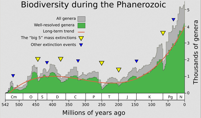
‘Everyone knows’ the ‘Big Five’ mass extinctions: at the ends of the Ordovician (a loss of 85% of species at ~444 Ma); Devonian (70% of species at ~369 Ma); Permian (81% of species at 252 Ma); Triassic (70% of species at 201 Ma); and Cretaceous (75% of species at 66 Ma) Periods. The magnitudes relate to marine life, the terrestrial fossil record being more incomplete and less reliable. And there have been many lesser bursts of extinction and evolutionary radiations that followed to replenish and further diversify life. Extinction peaks signify sudden environmental change for which several plausible ‘causes’ have been suggested: asteroid impact, LIPs, ocean anoxia and a few others involving astronomical factors. Biodiversity during the Phanerozoic was always in a state of flux, but with progressive increases after each major crisis to modern times. There are many physical or abiotic processes that may have influenced biodiversity. So there is much uncertainty in the interplay of cause and effect, in much the same way as fluctuations in the world economy since the Industrial Revolution are difficult to fathom, even though financial data are much more precise and limited. Fossil and environmental data are plagued by heterogeneity, irregular sampling and the uncertainties in geochronology and the largely geochemical proxies deployed to monitor past environmental change. Another factor is the plain fact that, as well as abiotic processes, life itself affects environments; again economics – e.g. the interplay of supply, demand and price – offers stark lessons about the reductionism that still dominates much scientific discourse.
A multinational group led by mathematician Ivan Sudakow of the Open University have analysed carbon and oxygen data from the last 539 Ma – the Phanerozoic Eon – to model how the link between the carbon cycle and Earth’s climate relates to the fossil record. Rather than trying to grapple with a reductionist approach, i.e. ‘cause and effect’, they have attempted to show how the ‘backdrop’ to evolution varied through time: how the Earth System was organised during the half-billion years of ‘visible life’ (Sudakow, I. Et al. 2026. Transitions between persistent climate–carbon regimes coincide with elevated Phanerozoic biosphere vulnerability. Nature Communications v. 17, article 7559; DOI: 10.1038/s41467-026-75655-9). They omit the 100 Ma-long Ediacaran Period (635 to 539 Ma) when tangible life was abundant, if primitive. A measure of biotic vulnerability derived from the fossil record is central to their comparative analysis. It conflates the turnover of genera with biotic diversity. The authors suggest that a high turnover at a time of low diversity indicates high vulnerability. The Ediacaran fauna is nowhere near as diverse as those following the Cambrian Explosion and simply vanished from the record at the end of the Neoproterozoic, hence its omission.

The methodology, data plots and language used by Sudakow et al. are pretty obscure for a general geological audience and thus for me! Be that as it may, their complex analysis leads them to suggest plausibly that climate and the carbon cycle remained in persistent states during five long periods: Cambrian–Upper Ordovician (539–447 Ma); Upper Ordovician–lowermost Carboniferous (447–358 Ma); Carboniferous–Middle Triassic (358–239 Ma). Middle Triassic–early Palaeogene (239–57 Ma); Post-Palaeogene (57–0 Ma). Biotic vulnerability fluctuated within them, the largest mass extinctions occurring when it rose to peaks towards the start and/or end of each persistent climate-carbon state. But their work grossly simplifies the vast complexity of interwoven biotic and abiotic processes. It leaves out global changes in sea-level, the varying supply of elements released to the oceans by continental weathering – nutrients (N, K, P and Fe), toxins (e.g. Hg and S) and skeleton-building elements (e.g. Si, Ca and Mg) – and fluctuations in dissolved oxygen that reflect varying redox conditions; to name but four. Each of them would impact on life in different ways, and each can be parameterised in detail by geochemical data from sedimentary rocks
So, a useful test for the authors’ hypothesis would be to perform the same kind of analysis using, for instance, well-documented sea-level changes since the Early Cambrian, which would have shifted the availability and location of ecological niches. Likewise, the course of super-continent accretion and break up. There are also Phanerozoic time series for the oxygenation of seawater, especially for deep-water sediments, which show irregular pulses of anoxia, some of which are implicated in extinctions such as the end-Permian. And there are more data that are relevant to the co-evolution of Earth and life. I would not be surprised if such studies produced different scenarios from those arising from investigations of just surface average temperature (SAT) and the carbon cycle. No doubt others will follow where Sudakow et al. have led. Perhaps that team has plans to diversify its approach.
A cautionary philosophical question, however, is, ‘How far can rationalisation, even using mathematically sophisticated methods, hope to unravel geological history and past fluctuations in the biosphere?’
The compendium of peer-reviewer comments and suggestions helped me to follow the logic of this somewhat arcane paper. Readers might also benefit from reading them.
See also: Shifts between stable climate-carbon states coincide with increased Phanerozoic biosphere vulnerability. Scienmag, 5 August 2026; Study of climate–carbon behaviour through the ages gives vital lessons on the earth’s capacity when under threat. Open University News, 30 July 2026