
The Cryogenian Period that lasted from 860 to 635 million years ago is aptly named, for it encompassed two maybe three episodes of glaciation. Each left a mark on every modern continent and extended from the poles to the Equator. In some way, this series of long, frigid catastrophes seems to have been instrumental in a decisive change in Earth’s biology that emerged as fossils during the following Ediacaran Period (635 to 541 Ma). That saw the sudden appearance of multicelled organisms whose macrofossil remains – enigmatic bag-like, quilted and ribbed animals – are found in sedimentary rocks in Australia, eastern Canada and NW Europe. Their type locality is in the Ediacara Hills of South Australia, and there can be little doubt that they were the ultimate ancestors of all succeeding animal phyla. Indeed one of them Helminthoidichnites, a stubby worm-like animal, is a candidate for the first bilaterian animal and thus our own ultimate ancestor. Using the index for Palaeobiology or the Search Earth-logs pane you can discover more about them in 12 posts from 2006 to 2023. The issue here concerns the question: Why did Snowball Earth conditions develop? Again, refresh your knowledge of them, if you wish, using the index for Palaeoclimatology or Search Earth-logs. From 2000 onwards you will find 18 posts: the most for any specific topic covered by Earth-logs. The most recent are Kicking-off planetary Snowball conditions (August 2020) and Signs of Milankovich Effect during Snowball Earth episodes (July 2021): see also: Chapter 17 in Stepping Stones.
One reason why Snowball Earths are so enigmatic is that CO2 concentrations in the Neoproterozoic atmospheric were far higher than they are at present. In fact since the Hadean Earth has largely been prevented from being perpetually frozen over by a powerful atmospheric greenhouse effect. Four Ga ago solar heating was about 70 % less intense than today, because of the ‘Faint Young Sun’ paradox. There was a long episode of glaciation (from 2.5 to 2.2 Ga) at the start of the Palaeoproterozoic Era during which the Great Oxygenation Event (GOE) occurred once photosynthesis by oxygenic bacteria became far more common than those that produced methane. This resulted in wholesale oxidation to carbon dioxide of atmospheric methane whose loss drove down the early greenhouse effect – perhaps a narrow escape from the fate of Venus. There followed the ‘boring billion years’ of the Mesoproterozoic during which tectonic processes seem to have been less active. in that geologically tedious episode important proxies (carbon and sulfur isotopes) that relate to the surface part of the Earth System ‘flat-lined’. The plethora of research centred on the Cryogenian glacial events seems to have stemmed from the by-then greater complexity of the Precambrian Earth System.
Since the GOE the main drivers of Earth’s climate have been the emission of CO2 and SO2 by volcanism, the sedimentary burial of carbonates and organic carbon in the deep oceans, and weathering. Volcanism in the context of climate is a two-edged sword: CO2 emission results in greenhouse warming, and SO2 that enters the stratosphere helps reflect solar radiation away leading to cooling. Silicate minerals in rocks are attacked by hydrogen ions (H+) produced by the solution of CO2 in rain water to form a weak acid (H2CO3: carbonic acid). A very simple example of such chemical weathering is the breakdown of calcium silicate:
CaSiO3 + 2CO2 + 3H2O = Ca2+ + 2HCO3– + H4SiO4
The reaction results in calcium and bicarbonate ions being dissolved in water, eventually to enter the oceans where they are recombined in the shells of planktonic organisms as calcium carbonate. On death, their shells sink and end up in ocean-floor sediments along with unoxidised organic carbon compounds. The net result of this part of the carbon cycle is reduction in atmospheric CO2 and a decreased greenhouse effect: increased silicate weathering cools down the climate. Overall, internal processes – particularly volcanism – and surface processes – weathering and carbonate burial – interact. During the ‘boring billion’ they seem to have been in balance. The two processes lie at the core of attempts to model global climate behaviour in the past, along with what is known about developments in plate tectonics – continental break-up, seafloor spreading and orogenies – and large igneous events resulting from mantle plumes. A group of geoscientists from the Universities of Sydney and Adelaide, Australia have evaluated the tectonic factors that may have contributed to the first and longest Snowball Earth of the Neoproterozoic: the Sturtian glaciation (717 to 661 Ma) (Dutkiewicz, A. et al. 2024. Duration of Sturtian “Snowball Earth” glaciation linked to exceptionally low mid-ocean ridge outgassing. Geology, v. 52, online early publication; DOI: 10.1130/G51669.1).

Shortly before the Sturtian began there was a major flood volcanism event, forming the Franklin large igneous province, remains of which are in Arctic Canada. The Franklin LIP is a subject of interest for triggering the Sturtian, by way of a ‘volcanic winter’ effect from SO2 emissions or as a sink for CO2 through its weathering. But both can be ruled out as no subsequent LIP is associated with global cooling and the later, equally intense Marinoan global glaciation (655 to 632 Ma) was bereft of a preceding LIP. Moreover, a world of growing frigidity probably could not sustain the degree of chemical weathering to launch a massive depletion in atmospheric CO2. In search of an alternative, Adriana Dutkiewicz and colleagues turned to the plate movements of the early Neoproterozoic. Since 2020 there have been two notable developments in modelling global tectonics of that time, which was dominated by the evolution of the Rodinia supercontinent. One is based largely on geological data from the surviving remnants of Rodinia (download animation), the other uses palaeomagnetic pole positions to fix their relative positions: the results are very different (download animation).
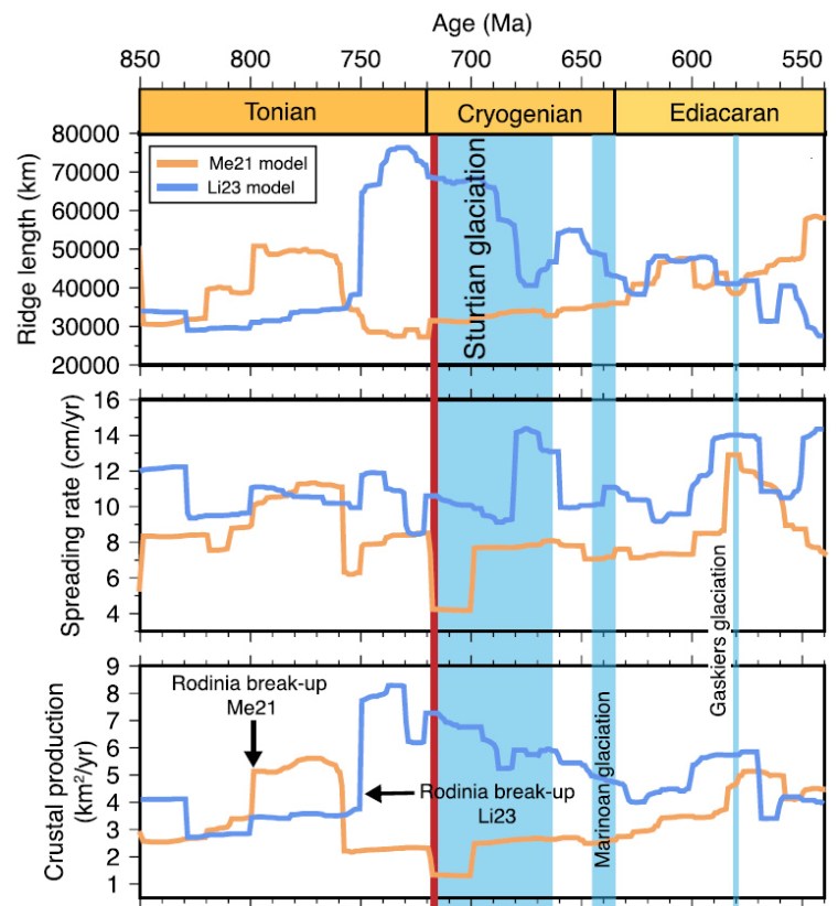
The geology-based model has Rodinia beginning to break up around 800 Ma ago with a lengthening of global constructive plate margins during disassembly. The resulting continental drift involved an increase in the rate of oceanic crust formation from 3.5 to 5.0 km2 yr-1. Around 760 Ma new crust production more than halved and continued at a much slowed rate throughout the Cryogenian and the early part of the Ediacaran Period. The palaeomagnetic model delays breakup of the Rodinia supercontinent until 750 Ma, and instead of the rate of crust production declining through the Cryogenian it more than doubles and remains higher than in the geological model until the late Ediacaran. The production of new oceanic crust is likely to govern the rate at which CO2 is out-gassed from the mantle to the atmosphere. The geology-based model suggests that from 750 to 580 Ma annual CO2 additions could have been significantly below what occurred during the Pleistocene ice ages since 2.5 Ma ago. Taking into account the lower solar heat emission, such a drop is a plausible explanation for the recurrent Snowball Earths of the Neoproterozoic. On the other hand, the model based on palaeomagnetic data suggests significant warming during the Cryogenian contrary to a mass of geological evidence for the opposite.
A prolonged decrease in tectonic activity thus seems to be a plausible trigger for global glaciation. Moreover, reconstruction of Precambrian global tectonics using available palaeomagnetic data seems to be flawed, perhaps fatally. One may ask, given the trends in tectonic data: How did the Earth repeatedly emerge from Snowball episodes? The authors suggest that the slowing or shut-down of silicate weathering during glaciations allowed atmospheric CO2 to gradually build up as a result of on-land volcanism associated with subduction zones that are a quintessential part of any tectonic scenario.
This kind of explanation for recovery of a planet and its biosphere locked in glaciation is in fact not new. From the outset of the Snowball Earth hypothesis much the same escape mechanisms were speculated and endlessly discussed. Adriana Dutkiewicz and colleagues have fleshed out such ideas quite nicely, stressing a central role for tectonics. But the glaring disparities between the two models show that geoscientists remain ‘not quite there’. For one thing, carbon isotope data from the Cryogenian and Ediacaran Periods went haywire: living processes almost certainly played a major role in the Neoproterozoic climatic dialectic.


