
Ocean floors, especially those of the Pacific and Indian oceans, are bespattered by tens of thousands of seamounts and volcano-based islands. Some of them define chains roughly aligned with the direction of sea-floor spreading and whose age of activity changes progressively along the chains. A few include bends linked to past changes in plate motions (see: The Great Bend of the Pacific Ocean Floor; May 2009). There are also vast, drowned plateaus, which mark oceanic equivalents of flood-basalt provinces on continents. The July 2026 issue of Nature Geoscience is dominated by four papers that are focused on such magmatism within oceanic plates, together with several commentaries and a striking cover image. The findings reported by the authors are briefly summarised by the Issue’s editor and two News & Views items (Editor 9 July 2026. Emerging insights on oceanic intraplate volcanism. Nature Geoscience v. 19, p. 739; DOI: 10.1038/s41561-026-02051-9; Ito, G. 2026. The deep link between intraplate volcanism and plate tectonics. Nature Geoscience v. 19, p. 743-744; DOI: 10.1038/s41561-026-02027-9. Whittaker, J. 2026. Linking plates to plumes in the Cretaceous Pacific. Nature Geoscience v. 19, p. 745-746: DOI: 10.1038/s41561-026-02026-w).

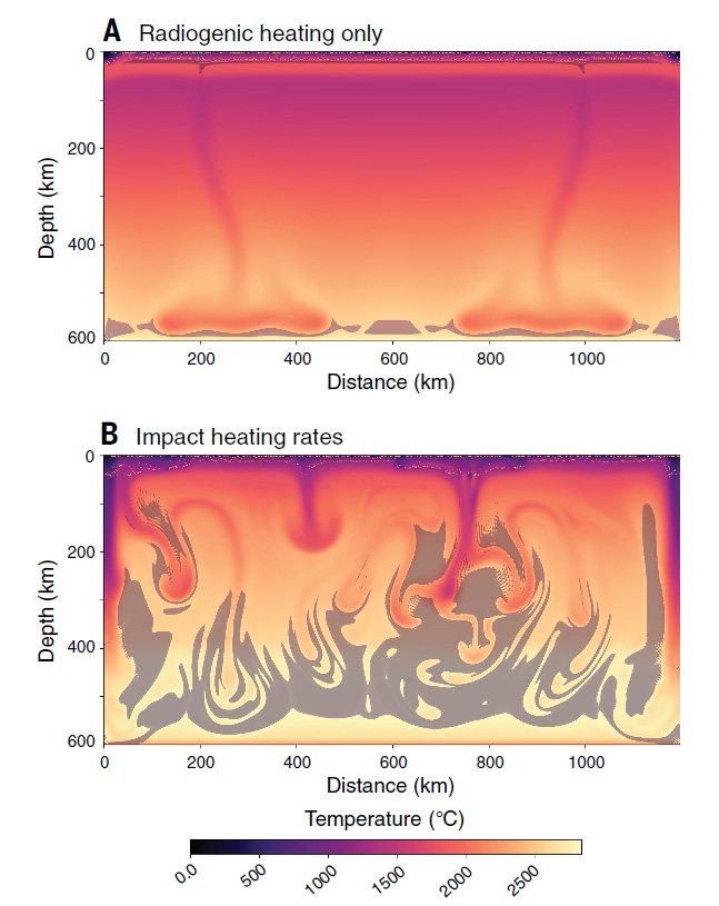
Age-progressive seamount chains have been ascribed since the birth of plate tectonics to the movement of an oceanic plate over ‘hot spots’ or mantle plumes. Yet the vast majority of sea mounts are apparently distributed at random. They have posed a bone of contention for oceanographers. One of the papers proposes a clear explanation (Hao Dong et al. 2026. Deep mantle plume origin of oceanic intraplate volcanism. Nature Geoscience v. 19, p. 828-836; DOI: 10.1038/s41561-026-02006-0. See also: Iyer, D, 2026 New 270‑Million‑Year Simulation Reveals Hidden Heat Zones Behind Thousands of Seamounts. Bioscience/Marine Science10 June 2026). The authors, based at the Institute of Geology and Geophysics of the Chinese Academy of Sciences, have produced a simulation of changing mantle dynamics beneath the Indian and Pacific Oceans over the last 290 Ma. In their model, hot mantle rising from the core-mantle boundary has repeatedly interacted with the oceanic upper mantle and lithosphere. This rise of hot mantle seems not always to manifest as discrete plumes from the depths. Rather it diffusely heats the asthenosphere to produce large-scale hot regions over which clusters of isolated seamounts formed while the thermal anomaly remained. They liken them to “seamount breweries”, and posit fragmentation of the rising mass of hot mantle, sometimes at depth or within the upper mantle. Such mechanisms drift with the overall mantle and lithospheric flow, so that seamount-volcanoes continue to develop, provided the ‘brewing zones’ retain sufficient heat.
But what might have launched such rising deep mantle? Another study notes that seamount volcanism is more voluminous on ocean floors that once passed over large low-shear-velocity provinces (LLSVPs) in the lowermost mantle beneath Africa and the Pacific Ocean (Conrad, C.P. & Domeier, M. Seamount volcanism associated with Earth’s basal mantle structures. Nature Geoscience v. 19, p. 822-827; DOI: 10.1038/s41561-026-02007-z) These massive deep-mantle provinces are hotter than their surroundings so they are less rigid, which is why seismic S-waves travel more slowly through them. They also lie on opposite sides of the Earth and may have done so for several billion years. Two other, independent studies in the same issue of Nature Geoscience also imply a connection to the deep mantle (Jinchang Zhang et al. 2026. Ontong Java Plateau formed by a thermochemical mantle plume. Nature Geoscience v. 19, p.846-854; DOI: 10.1038/s41561-026-02019-9; Dingshan Deng et al. 2026. Vigorous mantle convection triggered the Cretaceous Pacific large igneous provinces. Nature Geoscience v. 19, p. 837-845; DOI: 10.1038/s41561-026-02016-y).
Extrusion of large igneous provinces (LIPs) on the floor of the Pacific Ocean peaked during the Early Cretaceous. Dingshan Deng and colleagues modelled mantle flow that links subduction, plume activity and mid-ocean ridge activity, which suggests that deep-mantle upwelling peaked around 130 to 125 Ma ago and was driven by increased subduction around the ocean’s margin. This slowed down the rate of spreading at mid-ocean ridges so that heat had to be dissipated by increased melting elsewhere to outpour magma that created LIPs such as the Ontong Java Plateau. The article by Jinchang Zhang et al. focuses on the Ontong Java Plateau, the largest such volcanogenic structure known on Earth. Long regarded as having been produced by a huge buoyant, hot plume, they calculate that such a phenomenon would have had to have uplifted the ocean floor above sea level. That clearly did not happen. To reconcile the sheer volume of magma production with extrusion on deep ocean floor, the authors considered a denser and hotter source mantle, perhaps 135 to 200°C higher than ambient mantle temperature. One possibility is that it had incorporated a lot of older subducted slab materials and was hot enough to thermally erode the plate on which the Ontong Java Plateau was emplaved.
In the 70 years since ideas on plate tectonics began to develop the approach has changed. It began in a ‘compartmentalised’ fashion: spreading at mid-ocean ridges; descent at subduction zones; hot spots and mantle plumes, and so on. Most, if not all Earth scientists involved in this scientific revolution adhered to a reductionist philosophy; i.e. breaking down the hugely complex Earth system into simpler components – the whole is the sum of its parts – an approach begun in the 17th century by by René Descartes. Now, instead of a focus on and separation of cause and effect, it is becoming clearer that the Earth system is fundamentally one of global interconnections, in continuous motion and change. A change in one part inescapably rebounds on all the others, so that the system continually evolves. The tools available to geoscientists have evolved too.


