End-Ordovician mass extinction, faunal diversification, glaciation and true polar wander

Enormous events occurred between 460 and 435 Ma around the mid-point of the Palaeozoic Era and spanning the Ordovician-Silurian (O-S) boundary. At around 443 Ma the second-most severe mass extinction in Earth’s history occurred, which eliminated 50 to 60% of all marine genera and almost 85% of species: not much less than the Great Dying at the end of the Permian Period. The event was accompanied by one of the greatest biological diversifications known to palaeontology, which largely replaced the global biota initiated by the Cambrian Explosion. Centred on the Saharan region of northern Africa, Late Ordovician glacial deposits also occur in western South America and North America. At that time all the current southern continents and India were assembled in the Gondwana supercontinent, with continental masses that became North America, the Baltic region, Siberia and South China not far off: all the components that eventually collided to form Pangaea from the Late Silurian to the Carboniferous.

The mass extinction has troubled geologists for quite a while. There are few signs of major volcanism having been involved, although some geochemists have suggested that very high mercury concentrations in some Late Ordovician marine sediments bear witness to large, albeit invisible, igneous events. No large impact crater is known from those times, although there is a curious superabundance of extraterrestrial debris, including high helium-3, chromium and iridium concentrations, preserved in earlier Ordovician sedimentary rocks, around the Baltic Sea. Another suggestion, poorly supported by evidence, is destruction of the atmospheric ozone layer by a gamma-ray burst from some distant but stupendous supernova. A better supported idea is that the oceans around the time of the event lacked oxygen. Such anoxia can encourage solution of toxic metals and hydrogen sulfide gas. Unlike other mass extinctions, this one was long-drawn out with several pulses.

The glacial epoch also seems implicated somehow in the mass die-off, being the only one known to coincide with a mass extinction. It included spells of frigidity that exceeded those of the last Pleistocene glacial maximum, with the main ice cap having a volume of from 50 to 250 million cubic kilometres. The greatest of these, around 445 Ma, involved a 5°C fall in global sea-surface temperatures and a large negative spike in δ13C in carbon-rich sediments, both of which lasted for about a million years. The complex events around that time coincided with the highest ever extinction and speciation rates, the number of marine species being halved in a short space of time: a possible explanation for the δ13 C anomaly. Yet estimates of atmospheric CO2 concentration in the Late Ordovician suggests it was perhaps 8–16 times higher than today; Earth should have been a warm planet then. One probable contributor to extreme glacial conditions has been suggested to be that the South Pole at that time was well within Gondwana and thus isolated from the warming effect of the ocean. So, severe glaciation and a paradoxical combination of mass extinction with considerable biological diversification present quite an enigma.

A group of scientists based in Beijing, China set out to check the palaeogeographic position of South China between 460 and 435 Ma and evaluate those in  O-S sediments at locations on 6 present continents (Jing, X., Yang, Z., Mitchell, R.N. et al. 2022. Ordovician–Silurian true polar wander as a mechanism for severe glaciation and mass extinction. Nature Communications, v. 13, article 7941; DOI: 10.1038/s41467-022-35609-3). Their key tool is determining the position of the magnetic poles present at various times in the past from core samples drilled at different levels in these sedimentary sequences. The team aimed to test a hypothesis that in O-S times not only the entire lithosphere but the entire mantle moved relative to the Earth’s axis of rotation, the ‘slippage’ probably being at the Core-mantle boundary [thanks to Steve Rozario for pointing this out]. Such a ‘true polar wander’ spanning 20° over a mere  2 Ma has been detected during the Cretaceous, another case of a 90° shift over 15 Ma may have occurred at the time when Snowball Earth conditions first appeared in the Neoproterozoic around the time when the Rodinia supercontinent broke up and a similar event was proposed in 1994 for C-O times albeit based on sparse and roughly dated palaeomagnetic pole positions.

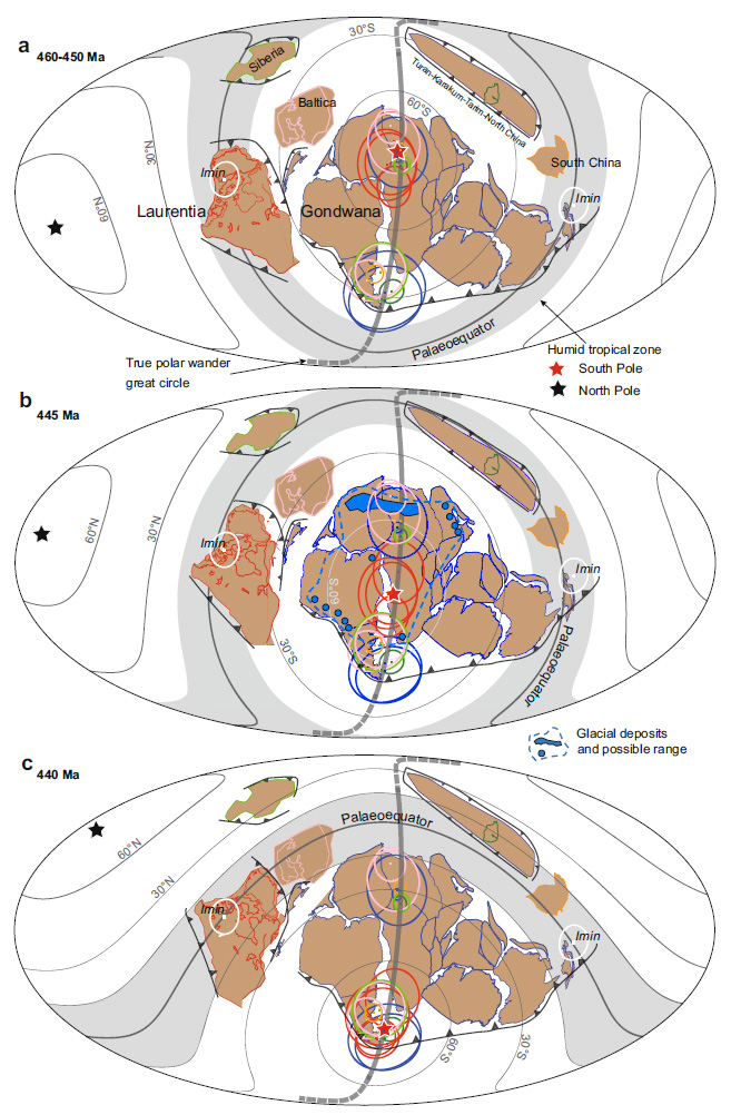
Xianqing Jing and colleagues report a wholesale 50° rotation of the lithosphere between 450 and 440 Ma that would have involved speeds of about 55 cm per year. It involved the Gondwana supercontinent and other continental masses still isolated from it moving synchronously in the same direction, as shown in the figure. From 460 to 450 Ma the geographic South Pole lay at the centre of the present Sahara. At 445 Ma its position had shifted to central Gondwana during the glacial period. By 440 Gondwana had moved further northwards so that the South Pole then lay at Gondwana’s southernmost extremity.

Palaeogeographic reconstructions charting true polar wander and the synchronised movement of all continental masses between 460 and 440 Ma. Note the changes in the trajectories of lines of latitude on the Mollweide projections. The grey band either side of the palaeo-Equator marks intense chemical weathering in the humid tropics. Credit Jing et al. Fig 5.

As well as a possible key to the brief but extreme glacial episode this astonishing journey by a vast area of lithosphere may help account for the mass extinction with rapid speciation and diversification associated with the O-S boundary. While the South Pole was traversing Gondwana as the supercontinent shifted the ‘satellite’ continental masses remained in or close to the humid tropics, exposed to silicate weathering and erosion. That is a means for extracting CO2 from the atmosphere and launching global cooling, eventually to result in glaciation over a huge tract of Gondwana around 445 Ma. Gondwana then moved rapidly into more clement climatic zones and was deglaciated a few million years later. The rapid movement of the most faunally diverse continental-shelf seas through different climate zones would have condemned earlier species to extinction simultaneous adaptation to changed conditions could have encouraged the appearance of new species and ecosystems. This does not require the catastrophic mechanisms largely established for the other mass extinction events. It seems that during the stupendous, en masse slippage of the Earth’s lithosphere plate tectonic processes still continued, yet it must have had a dynamic effect throughout the underlying mantle.

Yet the fascinating story does have a weak point. What if the position of the magnetic poles shifted during O-S times from their assumed rough coincidence with the geographic poles? In other words, did the self-exciting dynamo in the liquid outer core undergo a large and lengthy wobble? How the outer core’s circulation behaves depends on its depth to the solid core, yet the inner core seems only to have begun solidifying just before the onset of the Cambrian, about 100 Ma before the O-S events. It grew rapidly during the Palaeozoic, so the thickness of the outer core was continuously increasing. Fluid dynamic suggests that the form of its circulation may also have undergone changes, thereby affecting the shape and position of the geomagnetic field: perhaps even shifting its poles away from the geographic poles …

Environmental DNA reveals ecology in Northern Greenland from 2 Ma ago

The closest land to the North Pole is Peary Land in northern Greenland. Today, much of it is a polar desert and is bare of ice, so field geology is possible during the Arctic summer. It is one of the last parts of the northern hemisphere to have been mapped in detail. The bedrock ranges in age from the Mesoproterozoic to Upper Cretaceous, although the sequence is incomplete because of tectonic events and erosion during the Phanerozoic Eon. Its complex history has made Peary Land a draw for both structural geologists and stratigraphers. Apart from glacial tills the youngest rocks are estuarine sediments deposited in the early Pleistocene, between two glacial tills. They define one of the earliest known interglacials, roughly between 1.9 and 2.1 Ma, which lasted for an estimated 20 ka. Late Pliocene (3.4 Ma) sediments from around the Arctic Ocean have yielded rich fossil fauna and flora that suggest much warmer conditions – 10°C higher than those at present – before repeated glaciation began in the Northern Hemisphere. The sediments in Peary Land are fossiliferous, plant remains indicating a cover of coniferous trees, but animal fossils are restricted to small invertebrates: the tangible palaeontology offers slim pickings as regards assessing environmental conditions and the ecosystem.

One means of exploring faunal and floral diversity is through sampling and analysing DNA buried in sediments and soils rather than in fossils – plants shed pollen while animals spread their DNA via dung and urine. This approach has met with extraordinary success in revealing megafaunas that may have been decimated by humans newly arrived in the Americas. Even more remarkable was the ability of environmental DNA from cave sediments to reveal the former presence of individual humans who once lived in the caves and thus assess their numbers and relatedness. Such penetrating genetic ‘fingerprinting’ only became possible when new techniques to extract fragments of DNA from sediments and splice them to reconstruct genomes had been developed. But to apply them to material some two million years old would be a big ask; The oldest known DNA sequence had been recovered in 2021 from the molar of a 1.1 Ma old mammoth preserved in permafrost – a near-ideal source. A large multinational team under the supervision of Eske Willerslev (currently of Cambridge University, UK) took on the challenge, despite two million years of burial being likely to have degraded genetic material to minuscule fragments absorbed on the surface of minerals (Kjær, K.H. and 38 others 2022. A 2-million-year-old ecosystem in Greenland uncovered by environmental DNA. Nature, v 612, p. 283–291; DOI: 10.1038/s41586-022-05453-y). But it transpired that quartz grains have a good chance of ‘collecting’ bits of DNA and readily yielding them to the extraction media. The results are extraordinary.

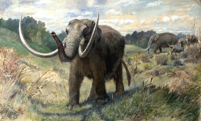
Reconstruction of an American mastodon herd by American painter of large extinct fauna Charles R. Knight

The DNA extraction turned-up signs of 70 vascular plants, including poplar, spruce and yew now typically found at much lower latitudes, alongside sedges, shrubs and birch-tree species that still grow in Greenland. The climate was substantially warmer than it is now. The fauna included elephants – probably mastodons (Mammut) but not mammoths (Mammuthus) and caribou, as well as rabbits, geese and various species of rodents. There were even signs of ants and fleas. The overall assemblage of plants has no analogue in modern vegetation, perhaps because of the absence of anthropogenic influences, such as fires, the smaller extent of glaciations, their shorter duration and less established permafrost during the early Pleistocene. The last factor could have allowed a quicker and wider spread of coniferous-deciduous woodland, found today in NE Canada. In turn this spread of vegetation would have drawn in herds of large herbivores, later mastodons being known to have been wide-ranging forest dwellers. Willerslev suggests that the study has a potential bearing on how ecosystems may respond to climate change.

Early land plants and oceanic extinctions

In September 2022 Earth-logs highlighted how greening of the continents affected the composition of the continental crust. It now seems that was not the only profound change that the first land plants wrought on the Earth system. Beginning in the Silurian, the spread of vegetation swept across the continents during the Devonian Period. From a height of less than 30 cm among the earliest species by the Late Devonian the stature of plants went through a large increase with extensive forests of primitive tree-sized conifers, cycads, horsetails and sporiferous lycopods up to 10 m tall. Their rapid evolution and spread was not hampered by any herbivores. It was during the Devonian that tetrapod amphibians emerged from the seas, probably feeding on burgeoning terrestrial invertebrates. The Late Devonian was marked by five distinct episodes of extinction, two of which comprise the Devonian mass extinction: one of the ‘Big Five’. This affected both marine and terrestrial organisms. Neither flood volcanism nor extraterrestrial impact can be linked to the extinction episodes. Rather they marked a long drawn-out period of repeated environmental stress.

Phytoplankton bloom off the east coast of Scotland ‘fertilised’ by effluents carried by the Tay and Forth estuaries.

One possibility is that a side effect of the greening of the land was the release of massive amounts of nutrients to the seas that would have resulted in large-scale blooms of phytoplankton whose death and decay depleted oxygen levels in the water column. That is a process seen today where large amounts of commercial fertilisers end up in water bodies to result in their eutrophication. Matthew Smart and others from Indiana University-Purdue University, USA and the University of Southampton, UK, geochemically analysed Devonian lake deposits from Greenland and Scotland to test this hypothesis (Smart, M.S. et al. 2022. Enhanced terrestrial nutrient release during the Devonian emergence and expansion of forests: Evidence from lacustrine phosphorus and geochemical records. Geological Society of America Bulletin, v. 134, early release article;  DOI: 10.1130/B36384.1).

Smart et al. show that in the Middle and Late Devonian the lacustrine strata show cycles in their abundance of phosphorus (P an important plant nutrient) that parallel evidence for wet and dry cycles in the lacustrine basins. The cycles show that the same phosphorus abundance patterns occurred at roughly the same times at five separate sites. This may suggest a climatic control forced by changes in Earth’s orbital behaviour, similar to the Milankovich Effect on the Pleistocene climate and at other times in Phanerozoic history. The wet and dry intervals show up in the changing ratio between strontium and copper abundances (Sr/Cu): high values signify wet conditions, low suggesting dry. The wet periods show high ratios of rubidium to strontium (Rb/Sr) that suggest enhanced weathering, while dry periods show the reverse – decreased weathering.

When conditions were dry and weathering low, P built up in the lake sediments, whereas during wet conditions P decreases; i.e. it was exported from the lakes, presumably to the oceans. The authors interpret the changes in relation to the fate of plants under the different conditions. Dry periods would result in widespread death of plants and their rotting, which would release their P content to the shallowing, more stagnant lakes. When conditions were wetter root growth would have increased weathering and more rainfall would flush P from the now deeper and more active lake basins. The ultimate repository of the sediments and freshwater, the oceans, would therefore be subject to boom and bust (wet and dry) as regards nutrition and phytoplankton blooms. Dead phytoplankton, in turn, would use up dissolved oxygen during their decay. That would lead to oceanic anoxia, which also occurred in pulses during the Devonian, that may have contributed to animal extinction.

See also: Linking mass extinctions to the expansion and radiation of land plants, EurekaAlert 10 November 2022; Mass Extinctions May Have Been Driven by the Evolution of Tree Roots, SciTechDaily, 14 November 2022.

Origin of animals at a time of chaotic oxygen levels

Every organism that you can easily see is a eukaryote, the vast majority of which depend on the availability of oxygen molecules. The range of genetic variation in a wide variety of eukaryotes suggests, using a molecular ‘clock’, that the first of them arose between 2000 to 1000 Ma ago. It possibly originated as a symbiotic assemblage of earlier prokaryote cells ‘bagged-up’ within a single cell wall: Lynn Margulis’s hypothesis of endosymbiosis. It had to have happened after the Great Oxygenation Event (GOE 2.4 to 2.2 Ga), before which free oxygen was present in the seas and atmosphere only at vanishingly small concentrations. Various single-celled fossil possibilities have been suggested to be the oldest members of the Eukarya but are not especially prepossessing, except for one bizarre assemblage in Gabon. The first inescapable sign that eukaryotes were around is the appearance of distinctive organic biomarkers in sediments about 720 Ma old. The Neoproterozoic is famous for its Snowball Earth episodes and the associated multiplicity of large though primitive animals during the Ediacaran Period (see: The rise of the eukaryotes; December 2017).

The records of carbon- and sulfur isotopes in Neo- and Mesoproterozoic sedimentary rocks are more or less flat lines after a mighty hiccup in the carbon and sulfur cycles that followed the GOE and the earliest recorded major glaciation of the Earth. The time between 2.0 and 1.0 Ga has been dubbed ‘the Boring Billion’. At about 900 Ma, both records run riot. Sulfur isotopes in sediments reveal the variations of sulfides and sulfates on the seafloor, which signify reducing and oxidising conditions respectively.  The δ13C record charts the burial of organic carbon and its release from marine sediments related to reducing and oxidising conditions in deep water. There were four major ‘excursions’ of δ13C during the Neoproterozoic, which became increasingly extreme. From constant anoxic, reducing conditions throughout the Boring Billion the Late Neoproterozoic ocean-floor experienced repeated cycles of low and high oxygenation reflected in sulfide and sulfate precipitation and by fluctuations in trace elements whose precipitation depends on redox conditions. By the end of the Cambrian, when marine animals were burgeoning, deep-water oxic-anoxic cycles had been smoothed out, though throughout the Phanerozoic eon anoxic events crop up from time to time.

Atmospheric levels of free oxygen relative to that today (scale is logarithmic) computed using combined carbon- and sulfur isotope records from marine sediments since 1500 Ma ago. The black line is the mean of 5,000 model runs, the grey area represents ±1 standard deviations. The pale blue area represents previous ‘guesstimates’. Vertical yellow bars are the three Snowball Earth events of the Late Neoproterozoic (Sturtian, Marinoan and Gaskiers). (Credit: Krause et al., Fig 1a)

The Late Neoproterozoic redox cycles suggest that oxygen levels in the oceans may have fluctuated too. But there are few reliable proxies for free oxygen. Until recently, individual proxies could only suggest broad, stepwise changes in the availability of oxygen: around 0.1% of modern abundance after the GOE until about 800 Ma; a steady rise to about 10% during the Late Neoproterozoic; a sharp rise to an average of roughly 80% at during the Silurian attributed to increased photosynthesis by land plants. But over the last few decades geochemists have devised a new approach based on variations on carbon and sulfur isotope data from which powerful software modelling can make plausible inferences about varying oxygen levels. Results from the latest version have just been published (Krause, A.J. et al. 2022. Extreme variability in atmospheric oxygen levels in the late Precambrian. Science Advances, v. 8, article 8191; DOI: 10.1126/sciadv.abm8191).

Alexander Krause of Leeds University, UK, and colleagues from University College London, the University of Exeter, UK and the Univerisité Claude Bernard, Lyon, France show that atmospheric oxygen oscillated between ~1 and 50 % of modern levels during the critical 740 to 540 Ma period for the origin and initial diversification of animals. Each major glaciation was associated with a rapid decline, whereas oxygen levels rebounded during the largely ice-free episodes. By the end of the Cambrian Period (485 Ma), by which time the majority of animal phyla had emerged, there appear to have been six such extreme cycles.

Entirely dependent on oxygen for their metabolism, the early animals faced periodic life-threatening stresses. In terms of oxygen availability the fluctuations are almost two orders of magnitude greater than those that animal life faced through most of the Phanerozoic. Able to thrive and diversify during the peaks, most animals of those times faced annihilation as O2 levels plummeted. These would have been periods when natural selection was at its most ruthless in the history of metazoan life on Earth. Its survival repeatedly faced termination, later mass extinctions being only partial threats. Each of those Phanerozoic events was followed by massive diversification and re-occupation of abandoned and new ecological niches. So too those Neoproterozoic organism that survived each massive environmental threat may have undergone adaptive radiation involving extreme changes in their form and function. The Ediacaran fauna was one that teemed on the sea floor, but with oxygen able to seep into the subsurface other faunas may have been evolving there exploiting dead organic matter. The only signs of that wholly new ecosystem are the burrows that first appear in the earliest Cambrian rocks. Evolution there would have ben rife but only expressed by those phyla that left it during the Cambrian Explosion.

There is a clear, empirical link between redox shifts and very large-scale glacial and deglaciation events. Seeking a cause for the dramatic cycles of climate, oxygen and life is not easy. The main drivers of the greenhouse effect COand methane had to have been involved, i.e. the global carbon cycle. But what triggered the instability after the ‘Boring Billion’? The modelled oxygen record first shows a sudden rise to above 10% of modern levels at about 900 Ma, with a short-lived tenfold decline at 800 Ma. Could the onset have had something to do with a hidden major development in the biosphere: extinction of prokaryote methane generators; explosion of reef-building and oxygen-generating stromatolites? How about a tectonic driver, such as the break-up of the Rodinia supercontinent? Then there are large extraterrestrial events … Maybe the details provided by Krause et al. will spur others to imaginative solutions. See also: How fluctuating oxygen levels may have accelerated animal evolution. Science Daily, 14 October 2022

Milankovich precession and the Palaeocene-Eocene Thermal Maximum

About 56 Ma ago there occurred some of the most dramatic biological changes since the mass extinction at the Cretaceous-Palaeogene boundary. They included rapid expansion and diversification of mammals and land plants, and a plunge in the number of deep-water foraminifera. Global cooling from the Cretaceous hothouse was rudely reversed by sudden global warming of about 5 to 10°C. Some climatologists have ascribed bugbear status to the Palaeocene-Eocene Thermal Maximum (PETM) as a possible scenario for future anthropogenic global warming. The widely accepted cause is a massive blurt into the Palaeocene atmosphere of greenhouse gases, but what caused it is enthusiastically debated. The climate shift is associated with a sudden decrease in the proportion of 13C in marine sediments: a negative spike in δ13C. Because photosynthesis favours the lighter 12C, organic matter has a low δ13C, so a great deal of buried organic carbon may have escaped from the ocean floor, most likely in the form of methane gas. However, massive burning of living terrestrial biomass would produce the same carbon-isotope signal, but absence of evidence for mass conflagration supports methane release. Methane is temporarily held in marine sediments in the form of gas hydrate (clathrate), an ice-like solid that forms at low temperatures on the deep seafloor. Warming of deep sea water or a decrease in pressure, if sea level falls, destabilise clathrates thereby releasing methane gas: the ‘clathrate gun hypothesis’. The main issue is what mechanism may have pulled the trigger for a monstrous methane release.

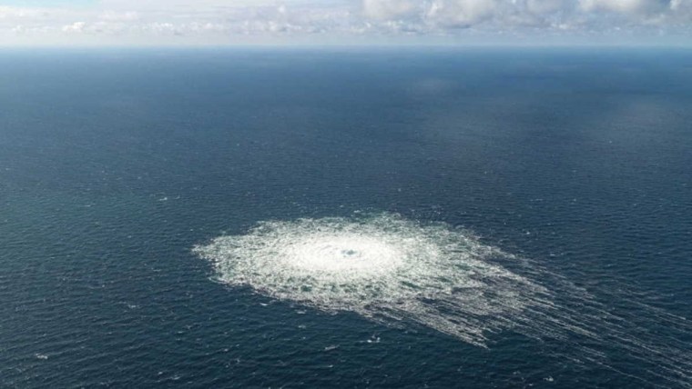
Massive leak of natural gas – mainly methane – off Sweden in the Baltic Sea, from the probably sabotaged Nord Stream pipeline. (Source: Swedish coastguard agency)

Many have favoured a major igneous event. Between 55.0 and 55.8 Ma basaltic magmatism– continuing today in Iceland – formed the North Atlantic Igneous Province. It involved large-scale intrusion of sills as well as outpourings of flood basalts and coincided with the initial rifting of Greenland from northern Europe (see: Smoking gun for end-Palaeocene warming: an igneous connection; July/August 2004). The occurrence of impact ejecta in end-Palaeocene sediments off the east coast of the US has spawned an extraterrestrial hypothesis for the warming, which could account for the negative spike in δ13C as the product of a burning terrestrial biosphere (see: Impact linked to the Palaeocene-Eocene boundary event; October 2016). Less headline-grabbing is the possibility that the event was part and parcel of the Milankovich effect: an inevitability in the complex interplay between the three astronomical components that affect Earth’s orbital and rotational behaviour: eccentricity, axial tilt and precession. A group of geoscientists from China and the US, led by Mingsong Li of Peking University, have investigated in minute detail the ups and downs of δ13C around 56 Ma in drill cores recovered from a sequence of Palaeocene and Eocene continental-shelf sediments in Maryland, USA (Li, M., Bralower, T.J. et al. 2022. Astrochronology of the Paleocene-Eocene Thermal Maximum on the Atlantic Coastal Plain. Nature Communications, v. 13, Article 5618; DOI: 10.1038/s41467-022-33390-x).

The study involved sampling sediment for carbon- and oxygen-isotope analysis at depth intervals between 3 and 10 cm over a 35 m section through the lower Eocene and uppermost Palaeocene. Calcium abundances in the core were logged at a resolution of 5 mm using an X-ray fluorescence instrument. The results link to variations in CaCO3 in the sediments across the PETM event. Another dataset involves semi-continuous measurements of magnetic susceptibility (MS) along the core. These measurements are able to indicate variations in delivery to the ocean of dissolved calcium and detrital magnetic minerals as climate and continental weathering vary through time. They are widely known to be good recorders of Milankovich cycles. After processing, the Ca and MS data sets show cyclical fluctuations relative to depth within the cores. ‘Tuning’ their frequencies to the familiar time series of Milankovich astronomical climate forcing reveals a close match to what would be expected if the climate fluctuations were paced by the 26 ka axial precession signal. My post of 17 June 2022 about the influence of precession over ‘iceberg armadas’ during the Pleistocene might be useful to re-read in this context. This correlation enabled the researchers to convert depth in the cores to time, so that the timing of fluctuations in carbon- and oxygen-isotope data that the PETM had created could be considered against various hypotheses for its cause. The ‘excursions’ of both began at the same time and reached the maxima of their changes from Palaeocene values over about 6,000 years. The authors consider that is far too long to countenance the release of methane as a result of asteroidal impact, or by massive burning of terrestrial vegetation. The other option that the beginning of the North Atlantic Igneous Province had been the trigger may also be ruled out on two grounds: the magmatism began earlier, and it continued for far longer. The onset of the PETM coincides with an extreme in precession-related climatic forcing. So Li et al. consider that a quirk in the Milankovich Effect could have played a role in triggering massive methane release. This might also explain features of the global calcium record in seafloor sediments as results of a brief period of ocean acidification during the PETM. Such an event would play havoc with carbonate-secreting organisms, such as foraminifera, by lowering the dissolved carbonate ion content on which they depend for their shells: hence their suffering considerable extinction. Of course, the other elements of astronomical forcing – eccentricity and axial tilt – would also have been operating on global climate at the time.  The long-term 100 and 405 ka eccentricity cycles may have played a role in amplifying warming, which may have resulted in increased burial of organic carbon and thus the amount of methane buried beneath the seabed.

A Lower Jurassic environmental crisis

Curiously, one of the largest environmental disruptions during the Phanerozoic Eon (i.e. since 541 Ma ago) does not stand out in the way that the ‘Big Five’ mass extinctions do. Each of them killed off between 70 and 95% of all marine species. The Jurassic was a period of biological recovery from the End-Triassic extinction 201 Ma ago. Throughout its ~50 Ma duration extinction rates were below the average for the Phanerozoic, and they remained relatively low until the K-Pg mass extinction that drew the Mesozoic Era to a close at 66 Ma. Nevertheless, there were significant extinctions, such as the demise of several lineages of herbivorous dinosaurs towards the end of the Early Jurassic followed by the rise of the familiar, long-necked variety of eusauropods. Marine organisms that secreted hard parts made of calcium carbonate also experienced a collapse then. From time to time during the Jurassic and Cretaceous Periods the oceans lost a great deal of dissolved oxygen, increasing the chances of organic carbon being buried in marine sediments. Such oceanic anoxia resulted in the widespread deposition of hydrocarbon source rocks in the form of black bituminous muds. Overall, both the Jurassic and Cretaceous experienced  greenhouse climatic conditions, with  atmospheric CO2 levels rising to almost 3000 ppm and oxygen levels significantly lower than the modern 21%. Sea levels rose by up to 200 metres, thought to be due to fast sea-floor spreading and large areas of warm, buoyant oceanic lithosphere.

A notable ocean-anoxia event took place during the Lower Jurassic, around 183 Ma ago at the start of the Toarcian Age. This stratigraphic level was penetrated by a 1.5 km borehole sunk in 2015-2016 at Mochras in North Wales, UK, on the shore of Cardigan Bay. The core provided the thickest and most complete record ever recovered for this event, and has been analysed in exquisite detail using many techniques. The most revealing data have been published by a multinational team led by scientists from Trinity College, Dublin (Ruhl, M. et al. 2022. Reduced plate motion controlled timing of Early Jurassic Karoo-Ferrar large igneous province volcanism. Science Advances, v. 8, article eabo0866; DOI: 10.1126/sciadv.abo0866).

Plate boundaries around Gondwanaland and the Karoo-Ferrar large igneous province in the Early Jurassic (small yellow dots show dated localities) . Large pink dots: positions of Tristan de Cunha and Bouvet hotspots at the time (Credit: Ruhl et al. Fig 1A)

At the start of the Toarcian (183.7 Ma) the 187Os/186Os ratio of the samples begins to rise from 0.3 to almost 0.8 to fall back to 0.3 by 180.8 Ma. Osmium isotopes are a measure of continental weathering, and this ‘excursion’ surely signifies significant global warming and increases in atmospheric humidity and acidity that broke down rocks at the continental surface. Over the same period δ13C rises, decreases to by far the lowest value in the Lower Jurassic, rises again to gradually fall back. The start of the Toarcian seems to have experienced a major release of carbon then a profound sequestration of organic carbon, presumably through burial of dead organisms in the black mudstones that signify anoxic conditions. Remarkably, the 95 m thick Toarcian black-mudstone sequence also reveals a tenfold increase in its content of the element mercury, from 20 to 200 parts per billion (ppb), peaking at the same time (~182.8 Ma) as the most negative δ13C value was reached: the acme of carbon sequestration. A coincidence of massive organic carbon burial and increased mercury in marine sediments also happened at the time of the end-Permian mass extinction, although that does not necessarily imply exactly the same mechanism.

The early Toarcian geochemical trends, however, coincide with the initiation and duration of the Karoo-Ferrar large igneous province, which formed flood basalts, igneous dyke swarms and large volcanic centres in South Africa and Antarctica. That LIP may have emitted mercury, but so too may have increased chemical weathering of the land surface. Whichever, mercury forms an organic compound (methyl mercury) in water bodies. Readily incorporated into living organisms, that could explain the close parallel between the δ13C and Hg records in the Jurassic sediment core from Wales. The Karoo-Ferrar igneous activity itself presents a bit of a conundrum, as suggested by Ruhl et al. It happened at the very time that there was a 120° change in the direction of motion of the tectonic plate carrying along Africa and, indeed, the Gondwanaland supercontinent during the Jurassic. The directional change also involved local plate movement stopping for a while. According to the authors, it wasn’t a fortuitous coincidence of two mantle plumes from the core-mantle boundary hitting the bottom of the continental lithosphere below Africa and Antarctica at this tectonic ‘U-turn’. It is more likely that the pause gave existing plumes the opportunity and time to ‘erode’ the base of the continental lithosphere and rise. Decompression melting would then have produced the voluminous magmas. The two plumes were in place for a very long time and created seamount chains as plates moved over them. Both are still volcanically active: Tristan de Cunha on the mid-Atlantic Ridge, and Bouvet Island at a triple junction between South Africa and Antarctica.

So, a venture to unravel a period of profound environmental change during the Early Jurassic, which didn’t result in mass extinction, may well have spawned a new model for massive igneous events that did. Ruhl et al. suggest that the short-lived Siberian, North Atlantic and East African Rift LIPs each seem to have coincided with short episodes of tectonic slowing-down: LIPs may result in dramatic environmental change, but at the whim of plate tectonics.

See also: https://scitechdaily.com/surprising-discovery-shows-how-slowing-of-continental-plate-movement-controlled-earths-largest-volcanic-events/

Climate out of control after the Permian-Triassic mass extinction

The snuffing out of up to 90 percent of all terrestrial and marine species at the end of the Permian (252 Ma) was the outcome of lethal climatic warming. It probably stemmed from a stupendous episode of flood basalt volcanism and intrusions in what is now Siberia that burned vast amounts of peat or coal in the basin that the flows filled (see: Coal and the end-Permian mass extinction; March 2011). The carbon dioxide so released created planetary hyperthermia and toxic acid rain. For at least five million years Earth was an almost sterile world, a notable absence being dense vegetation on the land surface – the Early Triassic is devoid of coal, whereas there is plenty of Late Permian age. Much the same slow recovery of life is found in meagre collections of land and marine animal fossils of that age. Yet, other mass extinctions were followed by recovery and species diversification at a much faster pace.

One conceivable explanation could be the near absence of vegetation whose photosynthesis and burial would otherwise draw down CO2 and the same goes for its marine equivalent phytoplankton. But there is a powerful inorganic means of carbon sequestration: silicate weathering. The chemistry depends on carbon dioxide dissolved in water. For simple silicates it can be expressed as:

2CO2 + H2O + CaSiO3 → Ca2+ + 2HCO3 + SiO2.

The higher the ambient temperature, the faster such reactions proceed. Most silicates are more complex and many common ones, such as feldspars, include aluminium, so that another product of weathering is insoluble, fine-grained clay minerals. So various soluble metal ions (Ca, Mg, K, Na etc), dissolved bicarbonate ions, silica in various guises and clays eventually end up in the sea. Once there, it is possible for them to recombine, as for instance calcium and bicarbonate ions:

Ca2+ + 2HCO3→ CaCO3 + CO2 + H2O

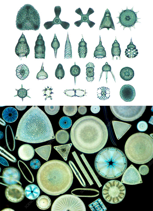
Despite some CO2 gas being released, this reaction results in a net sequestration of carbon in calcium carbonate. Incidentally, the same kind of chemical reaction occurs in the soils produced by weathering. The carbonate may cement soils to form a hard crust of caliche or ‘calcrete’. Chemical weathering enhanced by a hot climate, it might seem, should reduce the greenhouse effect quickly: a feedback mechanism that normally stabilises climate. But that did not happen after the P-Tr extinction event, thereby stressing all remaining life forms. A group of scientists at the University of Waikato in New Zealand have developed a possible explanation for this potentially fatal hazard for life on Earth (Isson, T.T. et al. 2022. Marine siliceous ecosystem decline led to sustained anomalous Early Triassic warmth. Nature Communications, v. 13, article 3509; DOI: 10.1038/s41467-022-31128-3). It focuses on the silica (SiO2) released by chemical weathering, which enters the ocean in the form of a colloid: Si(OH)4, a form of silicic acid known as ‘reactive silica’. Under ‘normal’ conditions, this is removed by organisms, such as diatoms and radiolaria, and is constantly recycled on a time scale of about 400 years, some contributing to deep-ocean oozes in the form of chert. But, like all other marine organisms, they too were victims of the P-Tr mass extinction.

Examples of marine radiolaria (top)

Reactive silica colloids in seawater also participate in inorganic chemical reactions, combining with dissolved metal ions to form complex hydrated aluminosilicates, i.e. more clay minerals. The reactions change the alkalinity of seawater. As a result dissolved HCO3ions transform to CO2 gas and water. Despite the complexity of the chemistry that interweaves the carbon and silicon cycles, there is a simple conclusion. If the abundance of silica-secreting marine organisms falls drastically while continental weathering continues to deliver silica, clay-mineral formation on the ocean floor results in release of CO2 that reverses the effect of enhanced weathering and thus maintains hyperthermal conditions. The other outcome is that less chert and flint granules form Terry Isson and colleagues examined the varying proportion of chert in cores through Lower Triassic marine sediments. A ‘chert gap’characterises the 4 to 6 Ma following the P-Tr boundary event. This can be explained in part by extinction of silica-secreting organisms and by inorganic reactions converting the reactive silica that enhanced weathering delivered to the oceans to clay minerals. This supports the idea that the inorganic part of the silica cycle maintained greenhouse conditions in the absence of organic ‘competition’ for reactive silica. Many other biogeochemical cycles link biological and chemical processes that combine to affect climate: involving phosphorus, nitrogen and iron, to name but three.

A new twist to Pleistocene climate cycles

The combined gravitational pulls of the sun and moon modulate variations in local tidal range. High spring tides occur when the two bodies are opposed at full moon or in roughly the same direction at new Moon. When the positions of sun and moon are at right angles (1st quarter and 3rd quarter) their gravitational pulls partly cancel each other to give neap tides. Consequently, there are two tidal cycles every lunar month.  In a similar way, the varying gravitational pulls of the planets during their orbital cycles impart a repetitive harmony to Earths astronomical behaviour. But their combined effects are on the order of tens of thousand years. Milutin Milankovich (1879-1958), a Serbian engineer, pondered on the possible causes of Earth’s climatic variations, particularly the repetition of ice ages. He was inspired by 19th century astronomers’ suggestion that maybe the gravitational effects of other planets might be a fruitful line of research. Milankovich focussed on how the shape of Earth’s orbit, the tilt of its rotational axis and the way the axis wobbles like that of a spinning top affect the amount of solar heating at all points on the surface: the effects of varying eccentricity, obliquity and precession, respectively.

 Earlier astronomers had calculated cycles of gravitational effects on Earth of the orbits of Jupiter and Saturn of the three attributes of Earth’s astronomical behaviour and found periods of about 100, 41 and 23 thousand years (ka) respectively. The other 3 inner planets and the much more distant giants Uranus and Neptune also have gravitational effects on Earth, but they are negligible compared with those of the two nearest giant planets, because gravitation force varies with mass and inversely with the square of distance. Sadly, Milankovich was long dead when his hypothesis of astronomical climate forcing was verified in 1976 by frequency analysis of the record of oxygen isotopes in foraminifera found in two ocean sediment core from the Southern Indian Ocean. It revealed that all three periods interfered in complex ways during the Late Pleistocene, to dominate variations in sea-surface temperatures and the fluctuating volume of continental ice sheets for which δ18O is a proxy (see: Odds and ends about Milankovich and climate change; February 2017).

Precession of the axis of a spinning top and that of the Earth. At present the northern end of Earth’s axis points to what we now call the Pole Star. Around 11.5 ka from now it will point to the star Vega

This was as revolutionary for climatology as plate tectonics was for geology. We now know that in the early Pleistocene glacial-interglacial cycles were in lockstep with the 41 ka period of axial obliquity, and since 700 ka followed closely – but not perfectly – the 100 ka orbital eccentricity forcing. The transitional period between 1.25 and 0.7 Ma (the Mid-Pleistocene Transition or MPT) suggested neither one nor the other. Milankovich established that axial tilt variations have the greatest influence on solar heating, so the early 41 ka cycles were no surprise. But the dominance of orbital eccentricity on the last 700 ka certainly presented a puzzle, for it has by far the weakest influence on solar heating: 10 times less than those of axial obliquity and precession. The other oddity concerns the actual effect of axial precession on climate change. There are no obvious 23 ka cycles in the climate record, despite the precession signal being clear in frequency analysis and its effect on solar heating being almost as powerful as obliquity and ten times greater than that of orbital eccentricity. Precessional wobbling of the axis controls the time of year when one hemisphere or the other is closest to the Sun. At one extreme it will be the Northern and 11.5 ka later it will be the Southern. The times of solstices and equinoxes also change relative to the calendar that we use today.

There is an important, if obvious, point about astronomical forcing of climate. It is always there, with much the same complicated interactions between the factors: human activities have absolutely no bearing on them. Climatic ‘surprises’ are likely to continue!

Changes in ice-rafted debris (IRD) since 1.7 Ma in a sediment core from the North Atlantic (orange fill) compared with its oxygen-isotope (δ18O) record of changes in continental ice cover (blue fill). At the top are the modelled variations in 23 ka axial precession (lilac) and 41 ka obliquity (green). The red circles mark major interglacial episodes, blue diamonds show the onset of significant ice rafting and orange diamonds are terminations of ice-rafting (TIR). (Credit: Barker et al., Fig. 2)

Sea temperature and ice-sheet volume are not the only things that changed during the Pleistocene. Another kind of record from oceanic sediments concerns the varying proportion in the muddy layers of abnormally coarse sand grains and even small pebbles that have been carried by icebergs; they are known as ice-rafted debris (IRD). The North Atlantic Ocean floor has plenty of evidence for them appearing and disappearing on a layer-by-layer basis. They were first recognised in 1988 by an oceanographer called Helmut Heinrich, who proposed that six major layers rich in IRD in North Atlantic cores bear witness to iceberg ‘armadas’ launched by collapse, or ablation, at the front of surging ice sheets on Scandinavia, Greenland and eastern Canada. Heinrich events, along with Dansgaard-Oeschger events (rapid climatic warming followed by slower cooling) in the progression to the last glacial maximum have been ascribed to a variety of processes  operating on a ‘millennial’ scale. However, ocean-floor sediment cores are full of lesser fluctuations in IRD, back to at least 1.7 Ma ago. That record offers a better chance of explaining fluctuations in ice-sheet ablation. A joint European-US group has investigated their potential over the last decade or so (Barker, S. et al. 2022. Persistent influence of precession on northern ice sheet variability since the early Pleistocene. Science, v. 376, p. 961-967; DOI: 10.1126/science.abm4033). The authors noted that in each glacial cycle since 1.7 Ma the start of ice rafting consistently occurred during a time of decreasing axial obliquity. Yet the largest ablation events were linked to minima in the precession cycles. In the last 700 ka, such extreme events are associated with the terminations of each ice age.

In the earlier part of the record, the 41 ka obliquity ‘signal’ was sufficient to drive glacial-interglacial cycles, hence their much greater regularity and symmetry than those that followed the Mid-Pleistocene Transition. The earlier ice sheets in the Northern Hemisphere also had consistently smaller extents than those after the MPT. Although the records show a role for precession in pre-MPT times in the form of ice-rafting events, the lesser effect of precession on summer warming at higher latitudes, compared with that of axial obliquity, gave it no decisive influence. After 700 ka the northern ice sheets extended much further south – as far as 40°N in North America – where summer warming would always have been commensurately greater than at high northern latitudes. So they were more susceptible to melting during the increased summer warming driven by the precession cycles. When maximum summer heating induced by axial precession in the Northern Hemisphere coincided with that of obliquity the ice sheets as a whole would have become prone to catastrophic collapse.

It is hard to say whether these revelations have a bearing on future climate. Of course, astronomical forcing will continue relentlessly, irrespective of anthropogenic greenhouse gas emissions. Earth has been in an interglacial for the last 11.5 ka, since the Younger Dryas; i.e. about half a precession cycle ago. The combination of obliquity- and precession-driven influences suggest that climate should be cooling and has been since 6,000 years ago, until the Industrial Revolution intervened. Can the gravitational pull of the giant planets prevent a runaway greenhouse effect, or will human effects defy astronomical forces that continually distort Earth’s astronomical behaviour?

Climate and tectonics since 250 Ma

A central feature of the Earth’s climate system is the way that carbon bound in two gases – carbon dioxide (CO2) and methane (CH4) – controls the amount of incoming solar energy that is retained by the atmosphere. Indeed, without one or the other our home world would have been locked in frigidity since shortly after its formation: a sterile, ice-covered planet. The ‘greenhouse effect’ has been ever-present because the material from which the Earth accreted contained carbon as well as every other chemical element from hydrogen to uranium. Naturally reactive, it readily combines with hydrogen and oxygen to form methane and carbon dioxide, which would have escaped the inner Earth as gases to enter the earliest atmosphere as a ‘comfort blanket’, along with water vapour, another greenhouse gas.  Their combined effects have remained crudely balanced so that neither inescapable frigidity nor surface temperatures high enough to boil-off the oceans have ever occurred in the last 4.5 billion years. Earth has remained like the wee bear’s porridge in the Goldilocks story! Even so, global climate has fluctuated again and again from that akin to a steamy greenhouse, through long periods of moderation to extensive glacial conditions, including three that extended from pole-to-pole – ‘Snowball’ Earths –  during in the Precambrian. During the Phanerozoic the Earth has entered three long periods of generally low global temperatures, in the Ordovician, the Carboniferous and during the last 2.5 Ma  that allowed polar ice caps and sea-ice to extend a third of the way to the Equator. These were forced back and forth repeatedly by cyclical influences apparently triggered by astronomically controlled changes to Earth’s orbital and rotational parameters – the Milankovich Effect. Anthropogenic emissions of greenhouse gases in vast and increasing amounts now threaten to disrupt natural climate variation, effectively overthrowing the gravitational influences of distant giant planets that have controlled climate changes that shaped our own evolution since the genus Homo first emerged.

Bubbles of air trapped in cores through the ice sheets of Antarctica and Greenland record decreased volumes of land ice as CO2 content increased and the opposite during glacial episodes. Somehow in step with the astronomical forcing the Earth released greenhouse gas to warm the climate and drew it down to bring on cooling. Since all life forms are built from carbon-rich compounds and some extract it from the environment to build carbonate hard parts, climate and life on land and in the oceans are interlinked. In fact life and death are involved, because once dead organisms and their hard parts are buried before being oxidised in sediments on land, as in peat and ultimately coal, and on the ocean floors as limestones or carbonaceous mudstones, atmospheric carbon is sequestered. Exposed to acid water containing dissolved CO2 from the atmosphere or to oxygen, respectively, the two forms of carbon in solid form are released as greenhouse gas once more. Both take place when sedimentary deposits are exhumed as a result of erosion and tectonics. Another factor is the abundance of available nutrients, themselves released and distributed by erosion and agents of transportation. At present surface waters of the most distant parts of the oceans contains plenty of such nutrients, except for a vital one, dissolved iron. So they are wet ‘deserts’. It seems that during the much dustier times of glacial episodes iron in fine form reached far out into the world’s oceans so that phytoplankton at the base of the food chain ‘bloomed ‘and so did planktonic animals. Dead organisms ‘rained’ to the ocean floor so drawing down CO2 from the atmosphere and decreasing the greenhouse effect. The surface parts of the carbon and rock cycles are extremely complex and climatologists have yet to come to grips with modelling its future climates convincingly. Yet the carbon cycle and much deeper parts of the rock cycle are interwoven too.

Carbon in sedimentary rock can be heated by burial, and some can be subducted to great depths at destructive plate margins together. The same applies to in ocean-floor basalts that have been permeated by circulating sea water through hydrothermal circulation to form carbonates in the altered volcanic rock. In both cases carbon stored for hundreds of million years can be released by metamorphism in orogenic belts at zones of continental collision and deep below island arcs. Carbon from mantle depths that has never ‘seen the light of day’ is also added to the atmosphere when magmas form below oceanic constructive margins, hot spots and subduction zones, and where magmas flood the continental surface. Consequently, plate tectonics and deep mantle convection have surely played a long-term role in the evolution of our planet’s climate system. Geoscientists based in Australia and the UK have used geochemical data to reconstruct the stores of carbon in oceanic plates and thermodynamic modelling to track what may have happened to it and the climate through the last 250 Ma (Müller, R.D. et al. 2022. Evolution of Earth’s tectonic carbon conveyor belt. Nature, v. 605, p. 629-639; DOI: 10.1038/s41586-022-04420-x). Their review is an important step in understanding what underpins climate on a geological time scale, onto which much shorter-term surface influences are superimposed.

The amount of carbon being outgassed as CO2 each year along plate boundaries in the early Jurassic (185 Ma) shown in dark purple (low) to yellow (high). Also shown in shades of blue is the accumulation of carbon stored in each square metre of the ocean plates. Plate motions are shown as grey arrows (credit: Müller, R.D. et al. Clip from video in Supplementary Information)

At mid-ocean ridges basaltic magma wells up from mantle depths and loses much of its content of dissolved CO2. The annual outgassing at ridges, which depends on the global rate of plate formation, has varied from 13 to 30 million tonnes of carbon  (MtC yr-1) since the start of the Mesozoic Era 250 Ma ago. Similarly, there is greenhouse-gas escape from volcanic arcs above subduction zones, estimated to have ranged from 0 to 18 MtC yr-1. As an oceanic plate moves away from its source various processes sequester CO2 into the oceanic crust and upper mantle through accumulation of deep-sea sediments and hydrothermal alteration of basaltic crust and peridotite mantle (ranging from 30 to 311 MtC yr-1). Of this influx of carbon into oceanic plates between 36 to 103 MtC yr-1 has gone down subduction zones in descending slabs. Between 0 to 49 MtC yr-1 of that has been outgassed by arc volcanic activity or absorbed into the overriding plate. The rest continues down into the deep mantle, perhaps to form diamonds. Overall, when the rate at which oceanic plates grow is rapid and plate motion speeds up, outgassing should be high. When plate growth slows, so does the rate of CO2 release. Variations in plate growth can be estimated from the magnetic reversal stripes above the ocean floors.  The authors have released an animation of the break-up of Pangaea (well worth watching at full screen – you can skip the ad at the start), with the rate of carbon emission at ridges and volcanic arcs being colour-coded. Also shown is the storage of carbon within oceanic plats plates as time passes.

Length of mid-ocean ridges (orange) and subduction zones (blue) through the last 250 Ma (top). The areas of oceanic crust produced at ridges and consumed by subduction (bottom) (credit: Müller, R.D. et al., Figs 1a, 1c)

Before Pangaea began to break up at the end of the Triassic (200 Ma) the total length of mid-ocean ridges was at a minimum of about 40 thousand km. Through the Jurassic it never exceeded 50,000 km, but rose to a maximum of 80,000 km during the Cretaceous then declined slowly to the current length of 60,000 km. Throughout the last 250 Ma the length of subduction zones stayed roughly the same at about 65 thousand km – not always in the same places – although the overall rate of subduction changed in line with the rate of oceanic plate growth  (the volume that is added must be balanced roughly by the amount that returns to the mantle).  Between the end of the Jurassic and the mid-Cretaceous crustal production and destruction doubled, shown by the bottom plot in the figure above. The very fast  movement of plates and an increase in the global length of ridges during Jurassic to mid-Cretaceous times led to a dramatic increase in CO2 outgassing from ridges so that its content in the atmosphere rose as high as 1200 ppm – more than four times that before the Industrial Revolution. That level resulted in global ‘hothouse’ conditions during the Cretaceous. Another factor behind the Cretaceous climate was a decrease in the global complement of mountains. That led to decreases in erosion and the weathering of silicates by acid rain, thus reducing natural sequestration of carbon.

During the Cenozoic (after 65 Ma) declining ridge outgassing was actually outpaced by that associated with subduction, according to the modelling. That is strange, for by around 35 Ma glaciation had begun  on Antarctica as the Earth was cooling, which implies a major, unexpected sink for excess CO2. The most likely way this might have arisen is through increased erosion and silicate weathering on the exposed continents that consumed CO2 faster than tectonics was releasing the gas. The length of continental arcs shows no sign of a major increase during the Cenozoic, which might have accelerated that kind of sequestration, but a variety of proxies for signs of weathering definitely suggests that there was an upsurge. Also there was increased storage of carbon on the deep ocean floor, shown by the video. Increased calcium released by weathering to enter ocean water in solution would allow more planktonic organisms to secrete calcite (CaCO3) skeletons that would then fall to the ocean floor when they died.

There may be more to be discovered in this hugely complex interplay between tectonics and climate. For instance, when the bottom waters of the oceans are oxygenated by deep currents of cold dense seawater sinking from polar regions, carbon in tissues of sunken dead organism is oxidised to release CO2. If bottom waters are anoxic, this organic carbon is preserved in sediments. The authors mention this as something to be considered in their future work on  the ‘tectonic carbon conveyor belt’.

The end of the Carboniferous ‘icehouse’ world

From about 340 to 290 Ma the Earth experienced the longest episode of repeated ice ages of the Phanerozoic. The climate then was similar in many ways to that of the Pleistocene. The South Polar region was then within the Pangaea supercontinent and thus isolated from any warming effect from the surrounding ocean: much the same as modern Antarctica but on a much larger scale. Glaciation extended as far across what became the southern continents and India as did the continental ice sheets of the Northern Hemisphere during Pleistocene glacial maxima. Tropical sedimentary rocks of the time, display evidence for repeated alternations of high and low sea levels that mark cycles of glacial maxima and interglacial episodes akin to those of the Pleistocene. In fact they probably reflect the influence of changes in the Earth’s orbit and geometry of its axis of rotation very similar to those predicted by Milankovich from astronomical factors to explain Pleistocene climatic cycles. At the end of the Carboniferous what was an ‘ice-house’ world changed suddenly to its opposite – ‘greenhouse’ conditions – that persisted through the Mesozoic Era until the later part of the Cenozoic, when Antarctica developed is ice cap and global climate slowly cooled to become extremely cyclical once again.

Sedimentary evidence for global climates 320 Ma ago. As well as the large tracts of glaciogenic sediments, smaller occurrences and examples of polished rock surfaces over which ice had passed show the probable full extent (blue line) of ice sheets across the southern, Gondwana sector of Pangaea (Credit: after Fig 7.3, S104, Earth and Space, ©Open University 2007)

The end of the Carboniferous witnessed the collapse of the vast Equatorial rainforests, which formed the coal deposits that put ‘Carbon’ into the name of the Period. By its end this ecosystem had vanished to result in a minor mass extinction of both flora and fauna. Temperatures rose and aridity set in, to the extent that the latest Carboniferous in the British coalfields is marked by redbeds that presage the spread of desert conditions across the Equatorial parts of Pangaea during the succeeding Permian. A team of researchers based at the University of California at Davis have been studying data pertaining to this sudden change have now published their findings (Chan J. and 17 others 2022. Marine anoxia linked to abrupt global warming during Earth’s penultimate icehouse. Proceedings of the National Academy of Sciences, v. 119, article e2115231119; DOI: 10.1073/pnas.2115231119). They used carbon-, oxygen- and uranium isotopes, together with proxies for changes in atmospheric CO2 concentrations, to model changes in the carbon cycle in the Late Carboniferous of China.

Changes in uranium isotopes within marine carbonates are useful indicators of the amount of oxygen available in ocean water at the sea floor. Between 304 and 303.5 Ma ago oxygen content declined by around 30%, the peak of this anoxia being at 303.7 Ma. This occurred about 100 ka after atmospheric CO2 had risen to ~700 parts per million (ppm) from around 350 ppm in the preceding 300 ka, as marked by several proxies.  The authors suggest that the lower ‘baseline’ for the main greenhouse gas marked an extreme glacial maximum. Changes in the proportions of 18O relative to ‘lighter’ 16O in fossil shells suggest that sea-surface temperatures increased in step with the doubling of the greenhouse effect. At the same time there was a major marine transgression as sea level rose. This would have been accompanied by a massive increase in low density freshwater in surface ocean water derived from melting of Pangaea’s ice cap. The team suggests that the freshened surface layer could not sink to carry oxygen to deeper levels, thereby creating anoxic conditions across an estimated 23% of the global seafloor, and thus toxic ‘death zones’ for marine organisms.

One possibility for this sudden rise of atmospheric CO2 is a massive episode of volcanism, perhaps a large igneous province, but there is scanty evidence for that at the end of the Carboniferous. A coinciding sharp decrease in δ13C  in carbonate shells suggests that the excess carbon dioxide probably had an organic origin. So a more plausible hypothesis is massive burning on the continental surface. In the tropics, the huge coals swamps would have contained vast amounts of peat-like decayed vegetable matter as well as living green vegetation. How might that have caught fire? The peat precursor to Carboniferous coal deposits derived from photosynthesis on an unprecedented, and never repeated, scale during tens of million years of thriving tropical rain forest during that Period. This built up atmospheric oxygen levels to about 35%, compared with about 21% today. Insects, whose maximum size is governed by their ability to take in oxygen through spiracles in their bodies, and by the atmospheric concentration of oxygen, became truly huge during the earlier Carboniferous. The more oxygen in the air, the greater the chance that organic matter will catch fire. In fact wet vegetation can burn if oxygen levels rise above 25%. At the levels reached in the Carboniferous huge wildfires in forests and peatlands would have been inevitable. Evidence that huge fires did occur comes from the amount of charcoal found in Carboniferous coal seams, which reach 70% compared with the 4 to 8 % in more recent coals. They may have been ignited by lightning strikes or even spontaneous combustion if decay of vegetation generated sufficient heat, as sometimes happens today in wet haystacks or garden compost heaps.  But how in a short period around 304 Ma could 9 trillion tons of carbon dioxide be released in this way. The preceding  glacial super-maximum, like glacial maxima of the Pleistocene, may have been accompanied by decreased atmospheric humidity: this would dry out the vast surface peat deposits.

The succeeding Permian is famous for its extensive continental redbeds, and so too those of the Triassic. They are red because sediment grains are coated in the iron oxide hematite (Fe2O3). As on Mars, the redbeds are a vast repository for oxygen sequestered from the atmosphere by the oxidation of dissolved Fe2+ to insoluble Fe3+. This had been going on throughout the Permian, the nett result being that by 250 Ma atmospheric oxygen content has slumped to 16% and remained so low for another 50 million years. Photosynthesis failed to resupply oxygen against this inorganic depletion, and there are few coal deposits of Permian or Triassic age: for about 100 Ma Earth ceased to have green continents.

See also: Carbon, climate change and ocean anoxia in an ancient icehouse world. Science Daily, 2 May 2022. 

‘Smoking gun’ for Younger Dryas trigger refuted

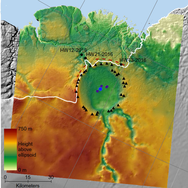
In 2018 airborne ice-penetrating radar over the far northwest of the Greenland revealed an impact crater as large as the extent of Washington DC, USA beneath the Hiawatha Glacier. The ice surrounding it was estimated to be younger than 100 ka. This seemed to offer a measure of support for the controversial hypothesis that an impact may have triggered the start of the millennium-long Younger Dryas episode of frigidity (12.9 to 11.7 ka). This notion had been proposed by a group of scientists who claimed to have found mineralogical and geochemical signs of an asteroid impact at a variety of archaeological sites of roughly this age in North America, Chile and Syria. A new study of the Hiawatha crater by a multinational team, including the original discoverers of the impact structure, has focussed on sediments deposited beyond the edge of the Greenland ice cap by meltwater streams flowing along its base. (Kenny, G.G. et al. 2022. A Late Paleocene age for Greenland’s Hiawatha impact structure. Science Advances, v.8, article eabm2434; DOI: 10.1126/science.eabm2434).

Colour-coded subglacial topography from airborne radar sounding over the Hiawatha Glacier of NW Greenland (Credit: Kjaer et al. 2018; Fig. 1D)

Where meltwater emerges from the Hiawatha Glacier downstream of the crater there are glaciofluvial sands and gravels that began to build up after 2010 when rapid summer melting began, probably due to global warming. As luck would have it, the team found quartz grains that contained distinctive planar features that are characteristic of impact shock. They also found pebbles of glassy impact melts that contain clasts of bedrock, further grains of shocked quartz and tiny needles of plagioclase feldspar that crystallised from the melt. Also present were small grains of the mineral zircon (ZrSiO4), both as pristine crystals in the bedrock clasts and porous, grainy-textured grains showing signs of deformation in the feldspathic melt rock. So, two materials that can be radiometrically dated are available: feldspars suitable for the 40Ar/39Ar method and zircons for uranium-lead (U-Pb) dating. The feldspars proved to be about 58 million years old; i.e. of Late Palaeocene age. The pristine zircon grains from bedrock clasts yielded Palaeoproterozoic U-Pb ages (~1915 Ma), which is the general age of the Precambrian metamorphic basement that underpins northern Greenland. The deformed zircon samples have a very precise U-Pb age of 57.99±0.54 Ma. There seems little doubt that the impact structure beneath the Hiawatha Glacier formed towards the beginning of the Cenozoic Era.

During the Palaeocene, Northern Greenland was experiencing warm conditions and sediments of that age show that it was covered with dense forest. The group that since 2007 has been advocating the influence of an impact over the rapid onset of the Younger Dryas acknowledges that the Hiawatha crater cannot support their view. But they have an alternative: an airburst of an incoming projectile. Although scientists know such phenomena do occur, as one did over the Tunguska area in Siberia on the morning of 30 June 1908. Research on the Tunguska Event has discovered  geochemical traces that may implicate an extraterrestrial object, but coincidentally the area affected is underlain by the giant SIberian Traps large igneous province that arguably might account for geochemical anomalies. Airbursts need to have been observed to have irrefutable recognition. Two posts from October 2021 – A Bronze Age catastrophe: the destruction of Sodom and Gomorrah? and Wide criticism of Sodom airburst hypothesis emerges – suggest that some scientists question the data used repeatedly to infer extraterrestrial events by the team that first suggested an impact origin for the Younger Dryas.

See also: Voosen, P, 2022. Controversial impact crater under Greenland’s ice is surprisingly ancient. Science, v. 375, article adb1944;DOI: 10.1126/science.adb1944

The Mid-Pleistocene Transition: when glacial cycles changed to 100 ka

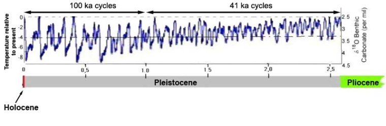
Before about a million years ago the Earth’s overall climate repeatedly swung from warm to cool roughly every 41 thousand years. This cyclicity is best shown by the variation of oxygen isotopes in sea-floor sediments. That evidence stems from the tendency during evaporation at the ocean surface for isotopically light  oxygen (16O) in seawater to preferentially enter atmospheric water vapour relative to 18O.  During cool episodes more water vapour that falls as snow at high latitudes fails to melt, so that glaciers grow. Continental ice sheets therefore extract and store 16O so that the proportion of the heavier 18O increases in the oceans. This shift shows up in the calcium carbonate (CaCO­3) shells of surface-dwelling organisms whose shells are preserved in sea-floor sediment. When the climate warms, the ice sheets melt and return the excess of 16O back to ocean-surface water, again marked by changed oxygen isotope proportions in plankton shells. The first systematic study of sea-floor oxygen isotopes over time revolutionised ideas about ancient climates in much the same way as sea-floor magnetic stripes revealed the existence of plate tectonics. Both provided incontrovertible explanations for changes observed in the geological record. In the case of oxygen isotopes climatic cyclicity could be linked to changes in the Earth’s orbital and rotational behaviour: the Milankovich Effect.

Glacial-interglacial cycles during the Pleistocene

The 41 ka cycles reflect periodic changes in the angle of the Earth’s rotational axis (obliquity), which have the greatest effect on how much solar heating occurs at high latitudes. However, between about 1200 and 600 ka the fairly regular, moderately intense 41 ka climate cycles shifted to more extreme, complex and longer 100 ka cycles at the ‘Mid-Pleistocene Transition’ (MPT). They crudely match cyclical variations in the shape of Earth’s orbit (eccentricity), but that has by far the least influence over seasonal solar heating. Moreover, modelling of the combined astronomical climate influences through the transition show little, if any, sign of any significant change in external climatic forcing. Thirty years of pondering on this climatic enigma has forced climatologists to wonder if the MPT was due to some sort of change in the surface part of the Earth system itself.

There are means of addressing the general processes at the Earth’s surface and how they may have changed by using other aspects of sea-floor geochemistry (Yehudai, M. and 8 others 2021. Evidence for a Northern Hemispheric trigger of the 100,000-y glacial cyclicity. Proceedings of the National Academy of Sciences, v. 118, article e2020260118; DOI: 10.1073/pnas.2020260118). For instance the ratio between the abundance of the strontium isotope 87Sr to that of 86Sr in marine sediments tells us about the progress of continental weathering around a particular ocean basin. The 87Sr/ 86Sr ratio is higher in rocks making up the bulk of the crystalline continental crust than that in basalts of the oceanic crust. That ratio is currently uniform throughout all ocean water. During the Cenozoic Era the ratio steadily increased in sea-floor sediments, reflecting the continual weathering and erosion of the continents. In the warm Pliocene (5.3 to 2.8 Ma) 87Sr/ 86Sr remained more or less constant, but began increasing again at the start of the Pleistocene with the onset of glaciation in the Northern Hemisphere. At about 1450 ka it began to increase more rapidly suggesting increased weathering, and then settled back to its earlier Pleistocene rate after 1100 ka. Another geochemical contrast between the continental and oceanic crust lies in the degree to which the ratio of two isotopes of neodymium (143Nd/144Nd) in rocks deviates from that in the Earth’s mantle – modelled from meteorite geochemistry – a measure signified by ЄNd. Magmatic rocks and young continental rocks have positive ЄNd values, but going back in time continental crust has increasingly negative ЄNd.

Yehudai et al analysed cores from deep-sea sediments that had been drilled between 41°N and 43°S in the Atlantic Ocean floor. They targeted layers designated as glacial and interglacial from their oxygen isotope geochemistry at different levels in the cores to check how ЄNd varied with time. The broad variations within each core look much the same, although at increasingly negative values from south to north, except in one case. The data from the most northerly Atlantic core show far more negative values of ЄNd, in both glacial and interglacial layers at around 950 ka ago, than do cores further to the south. The authors interpret this anomaly as showing a sudden increase in the amount of very old continental rocks – with highly negative ЄNd – that had become exposed at and ground from the base of the great northern ice sheets of North America, Greenland and Scandinavia. At present, the shield areas where the great ice sheets occurred until about 11 ka are almost entirely crystalline Precambrian basement, including the most ancient rocks that are known. Although broadly speaking the shields now have low relief, they are extremely rugged terrains of knobbly basement outcrops and depressions filled with millions of lakes. In the earlier Cenozoic they were covered by younger sedimentary rocks and soils formed by deep weathering, with less-negative ЄNd values. The authors conclude that around 950 ka that younger cover had largely been removed by glacial every every 41 ka or so since about 2.6 Ma ago, when glaciation of the Northern Hemisphere began.

The surface on which the North American ice sheet moved – typical Canadian Shield.

So what follows from that ЄNd anomaly? Yehudai et al suggest that in earlier Pleistocene times each successive ice sheet rested on soft rock; i.e. their bases were well lubricated. As a result, glaciers quickly reached the coast to break up and melt as icebergs drifted south. Exposure of the deeper, very resistant crystalline basement resulted in much more rugged base, as can be seen in northern Canada and Scandinavia today. Friction at their bases suddenly increased, so that much more ice was able to build up on the great shields surrounding the Arctic Ocean than had previously been possible. Shortly after 950 ka the sea-floor cores also reveal that deep ocean circulation weakened significantly in the following 100 ka. The influence on climate of regular, 41 ka changes in the tilt of the Earth’s rotational axis could therefore not be sustained in the later Pleistocene. The ice sheets could neither melt nor slide into the sea sufficiently quickly; indeed, bigger and more durable ice sheets would reflect away more solar heating than was previously possible as glacial gave way to interglacial. The 41 ka astronomical ‘pacemaker’ still operated, but ineffectually. A new and much more complex climate cyclicity set in. Insofar as climate change became stabilised, an overall ~100 ka pulsation emerged. Whether or not this fortuitously had the same pace as the weak influence of Earth’s changing orbital eccentricity remains to be addressed. The climate system just might be too complicated and sensitive for us ever to tell: it may even have little relevance in a climatically uncertain future.

See also: Why did glacial cycles intensify a million years ago? Science Daily, 8 November 2021.

Multiple impacts set back oxygen build-up in the Archaean

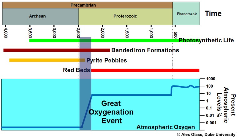
Earth’s present atmosphere contains oxygen because of one form of photosynthesis that processes water and carbon dioxide to make plant carbohydrates, leaving oxygen at a waste product. The photochemical trick that underpins oxygenic photosynthesis seems only to have evolved once. It was incorporated in a simple, single-celled organism or prokaryote, which lacks a cell nucleus but contains the necessary catalyst chlorophyll. Such an organism gave rise to cyanobacteria or blue-green bacteria, which still make a major contribution to replenishing atmospheric oxygen. Chloroplasts that perform the same function in plant cells are so like cyanobacteria that they were almost certainly co-opted during the evolution of a section of nucleus-bearing eukaryotes that became the ancestors of plants. A range of evidence suggests that oxygenic photosynthesis appeared during the Archaean Eon, the most tangible being the presence of stromatolites, which cyanobacteria mats or biofilms form today. These knobbly structures in carbonate sediments extend as far back as 3.5 billion years ago (see: Signs of life in some of the oldest rocks; September 2016). Yet it took a billion years before the first inklings of biogenic oxygen production culminated in the Great Oxygenation Event or GOE (see: Massive event in the Precambrian carbon cycle; January, 2012) at around 2400 Ma. Then, for the first time, oxidised iron in ancient soils turned them red. If oxygen was being produced, albeit in small amounts, in shallow, sunlit Archaean seas, why didn’t it build up in the atmosphere of those times? Geochemical analyses of Archaean sediments do point to trace amounts, with a few ‘whiffs’ of more substantial amounts. But they fall well below those of Meso- and Neoproterozoic and Phanerozoic times. One hypothesis is that Archaean oceans contained dissolved, ferrous iron (Fe2+) – a powerful reducing agent – with which available oxygen reacted to form insoluble ferric iron (Fe3+) oxides and hydroxides that formed banded iron formations (BIFS). The Fe2+ in this hypothesis is attributed to hydrothermal activity in basaltic oceanic crust. There is, however, another possibility for suppression of atmospheric oxygen accumulation in the Archaean and early-Palaeoproterozoic.

Summary of the evolution of atmospheric oxygen and related geological features. The percentage scale is logarithmic with the modern level being100%. Credit Alex Glass, Duke University

Simone Marchi of the Southwest Research Institute of Boulder, CO, USA and colleagues from the US, Austria and Germany suggest that planetary bombardment offers a plausible explanation (Marchi, S. et al 2021. Delayed and variable late Archaean atmospheric oxidation due to high collision rates on Earth. Nature Geoscience, v. 14 advance publication; DOI: 10.1038/s41561-021-00835-9). Over the last 20 years evidence of extraterrestrial impacts has emerged, in the form of thin spherule-bearing layers in Archaean sedimentary strata, probably formed by impacts of objects around 10 km across. So far 35 such layers have been identified from several locations in South Africa and Western Australia. They span the last billion years of the Archaean and the earliest Palaeoproterozoic, although they are not evenly spaced in time. The spherules represent droplets of mainly crustal but some meteoritic rocks that were vaporised by impacts and then condensed as liquid. Meteorites in particular contain reduced elements and compounds, including iron, whose oxidation by would remove free oxygen.

The evidence from spherule beds is supplemented by the team’s new calculations of the likely flux of impactors during the Archaean. These stem from re-evaluation of the lunar cratering record that is used to estimate the number and size of impacts on Earth up to 2.5 Ga ago. This flux amounts to the ‘leftovers’ of the catastrophic period around 4.1 Ga when the giant planets Jupiter and Saturn ran amok before they settled into their present orbits. Their perturbation of gravitational fields in the solar system injected a long-lived supply of potential impactors into the inner solar system, which is recorded by craters on the post-4.1 Ga lunar maria. The calculations suggest that the known spherule layers underestimate the true number of such collisions on Earth. Modelling by Marchi et al., based on the meteorite flux and the oxidation of vaporised materials produced by impacts, plausibly accounts for the delay in atmospheric oxygen build-up.

It is worth bearing in mind, however, that large impacts and their geochemical aftermath are, in a geological sense, instantaneous events widely spaced in time. They may have chemically ‘sucked’ oxygen out of the Archaean and early-Palaeoproterozoic atmosphere. Yet photosynthesising bacteria would have been generating oxygen continuously between such sudden events. The same goes for the supply of reduced ferrous iron and its circulation in the oceans of those times, capable of scavenging available oxygen through simple chemical reactions. In fact we can still observe that in action around ocean-floor hydrothermal vents where a host of reduced elements and compounds are oxidised by dissolved oxygen. The difference is that oxygen is now produced more efficiently on land and in the upper oceans and a less vigorous mantle is adding less iron-rich basalt magma to the crust: the balance has changed. Another issue is that the Great Oxygenation Event terminated the oxygen-starved conditions of the Archaean and Palaeoproterozoic in about 200 million years, despite the vast production of BIFs before and after it happened. The Wikipedia entry for the GOE provides a number of hypotheses for how that termination came about. Interestingly, one idea looks to a shortage of dissolved nickel that is vital for methane generating bacteria: a nickel ‘famine’. A geochemical setback for methanogens would have been a boost for oxygenic photosynthesisers and especially their waste product oxygen: methane quickly reacts with oxygen in the atmosphere to produce CO2 and water. Anomalously high nickel is a ‘signature element’ for meteorite bombardment, though it can be released by hydrothermal alteration of basalt. Had meteoritic nickel been fertilising methane-generating bacteria in the oceans prior to the GOE?

See also: A new Earth bombardment model. Science Daily, 21 October 2021.

Influence of massive igneous intrusions on end-Triassic mass extinction

About 200 Ma ago, the break-up of the Pangaea supercontinent was imminent. The signs of impending events are spread through the eastern seaboard of North America, West Africa and central and northern South America. Today, they take the form of isolated patches of continental flood basalts, dyke swarms – probably the feeders for much more extensive flood volcanism – and large intrusive sills. Break-up began with the separation of North America from Africa and the start of sea-floor spreading that began to form the Central Atlantic Ocean: hence the name Central Atlantic Magmatic Province (CAMP) for the igneous activity. It all kicked off at the time of the Triassic-Jurassic stratigraphic boundary, and a mass extinction with a similar magnitude to that at the end of the Cretaceous. Disappearances of animals in the oceans and on continents were selective rather than general, as were extinctions of land plants. The mass extinction is estimated to have taken about ten thousand years. It left a great variety of ecological niches ready for re-occupation. On land a small group of reptiles with a substantial destiny entered some of these vacant niches. They evolved explosively to the plethora of later dinosaurs as their descendants became separated as a result of continental drift and adaptive radiation.

Flood basalts of the Central Atlantic Magmatic Province in Morocco (Credit: Andrea Marzoli)

The end-Triassic mass extinction, like three others of the Big Five, was thus closely associated in time with massive continental flood volcanism: indeed one of the largest such events. Within at most 10 ka large theropod dinosaurs entered the early Jurassic scene of eastern North America. The Jurassic was a greenhouse world whose atmosphere had about five times more CO2, a mean global surface temperature between 5 and 10°C higher and deep ocean temperatures 8°C above those at present. Was mantle carbon transported by CAMP magmas the main source (widely assumed until recently) or, as during the end-Permian mass extinction, was buried organic carbon responsible? A multinational group of geoscientists have closely examined samples from a one million cubic kilometre stack of intrusive basaltic sills, dated at 201 Ma, in the Amazon basin of Brazil that amount to about a third of all CAMP magmatism (Capriolo, M. and 11 others 2021. Massive methane fluxing from magma–sediment interaction in the end-Triassic Central Atlantic Magmatic ProvinceNature Communications, v. 12, article 5534; DOI: 10.1038/s41467-021-25510-w).

The team focussed on fluid inclusions in quartz within the basaltic sills that formed during the late stages of their crystallisation. The tiny inclusions contain methane gas and tiny crystals of halite (NaCl) as well as liquid water. Such was the bulk composition of the intrusive magma that the presence of around 5% of quartz in the basalts would be impossible without their magma having assimilated large volumes of silica-rich sedimentary rocks such as shales. The host rocks for the huge slab of igneous sills are sediments of Palaeozoic age: a ready source for contamination by both organic carbon and salt. The presence of methane in the inclusions suggests that more complex hydrocarbons had been ‘cracked’ by thermal metamorphism. Moreover, it is highly unlikely to have been derived from the mantle, partly because methane has been experimentally shown not to be soluble in basaltic magmas whereas CO2 is. The authors conclude that both quartz and methane entered the sills in hydrothermal fluids generated in adjacent sediments. Thermal metamorphism of the sediments would also have driven such fluids to the surface to inject methane directly to the atmosphere. Methane is 25 times as potent as carbon dioxide at trapping heat in the atmosphere, yet it combines with the hydroxyl (OH) radical to form CO2 and water vapour within about 12 years. Nevertheless during continuous emission methane traps 84 times more heat in the atmosphere than would an equivalent mass of carbon dioxide.

Calculations suggest about seven trillion tonnes of methane were generated by the CAMP intrusions in Brazil. Had the magmas mainly been extruded as flood basalts then perhaps global warming at the close of the Triassic would have been far less. Extinctions and subsequent biological evolution would have taken very different paths; dinosaurs may not have exploded onto the terrestrial scene so dramatically during the remaining 185 Ma of the Mesozoic. So it seems important to attempt an explanation of why CAMP magmas in Brazil did not rise to the surface but stayed buried as such stupendous igneous intrusions. Work on smaller intrusive sills suggests that magmas that are denser than the rocks that they pass through – as in a large, thick sedimentary basin – are forced by gravity to take a lateral ‘line of least resistance’ to intrude along sedimentary bedding. That would be aided by the enormous pressure of steam boiled from wet sedimentary rocks forcing beds apart. In areas where only thin sedimentary cover rests on crystalline, more dense igneous and metamorphic rocks, basaltic magma has a greater likelihood of rising through vertical dyke swarms to reach the surface and form lava floods.

Anthropocene more an Event than an Epoch.

The Vattenfall lignite mine in Germany; the Anthropocene personified

The issue of whether or not to assign the time span during which human activities have been significantly affecting the planet and its interwoven Earth Systems has been dragging on since the term ‘Anthropocene’ was first proposed more than two decades ago. A suggestion that may resolve matters, both amicably and with a degree of scientific sense, has emerged in a short letter to the major scientific journal Nature, written by six eminent scientists (Bauer, A.M. et al. 2021. Anthropocene: event or epoch? Nature, v. 597, p. 332; DOI: 10.1038/d41586-021-02448-z). The full text is below

The concept of the Anthropocene has inspired more than two decades of constructive scholarship and public discussion. Yet much of this work seems to us incompatible with the proposal to define the Anthropocene as an epoch or series in the geological timescale, with a precise start date and stratigraphic boundary in the mid-twentieth century. As geologists, archaeologists, environmental scientists and geographers, we have another approach to suggest: recognize the Anthropocene as an ongoing geological event.

The problems with demarcating the Anthropocene as a globally synchronous change in human–environment relations, occurring in 1950 or otherwise, have long been evident (P. J. Crutzen and E. F. Stoermer IGBP Newsletter 41, 17–18; 2000). As an ongoing geological event, it would be analogous to other major transformative events, such as the Great Oxidation Event (starting around 2.4 billion years ago) or the Great Ordovician Biodiversification Event (around 500 million years ago).

Unlike formally defined epochs or series, geological events can encompass spatial and temporal heterogeneity and the diverse processes — environmental and now social — that interact to produce global environmental changes. Defining the Anthropocene in this way would, in our view, better engage with how the term has been used and criticized across the scholarly world.”

AUTHORS: Andrew M. Bauer, Stanford University, Stanford, California, USA; Matthew Edgeworth, University of Leicester, Leicester, UK;  Lucy E. Edwards, Florence Bascom Geoscience Center, Reston, Virginia, USAErle C. Ellis, University of Maryland, Baltimore County, Maryland, USA ; Philip Gibbard, Scott Polar Research Institute, University of Cambridge, Cambridge, UK;  Dorothy J. Merritts, Franklin and Marshall College, Lancaster, Pennsylvania, USA.

I have been grousing about the attempt to assign Epoch/Series status to the Anthropocene for quite a while (you can follow the development of my personal opinions by entering ‘Anthropocene’ in the Search Earth-logs box). In general I believe that the proposal being debated is scientifically absurd, and a mere justification for getting a political banner to wave. What the six authors of this letter propose seems eminently sensible. I hope it is accepted by International Commission on Stratigraphy as a solution to the increasingly sterile discussions that continue to wash to and fro in our community. Then perhaps the focus can be on action rather than propaganda.

As things have stood since 21 May 2019, a proposal to accept the Anthropocene as a formal chrono-stratigraphic unit defined by a GSSP at its base around the middle of the 20th century is before the ICS and the International Union of Geological Sciences (IUGS) for ratification. It was accepted by 88% of the 34-strong Anthropocene Working Group of the ICS Subcommission on Quaternary Stratigraphy. But that proposal has yet to be ratified by either the ICS or IUGS. Interestingly, one of the main Anthropocene proponents was recently replaced as chair of the Working Group.

When Greenland was a warm place

On 14-15 August 2021 it rained for the first time since records began at the highest point on the Greenland ice cap. Summit Camp at 3.216 m is run by the US National Science Foundation, which set it up in 1989, and is famous for climate data gleaned from two deep ice cores there. This odd event came at a time when surface melting of the ice cap covered 870 thousand km2: over half of its total 1.7 million km2 extent: a sure sign of global warming. The average maximum temperature in August at Summit is -14°C, but since the mid 20th century the Arctic has been warming at about twice the global rate. Under naturally fluctuating climatic conditions during the Pleistocene, associated with glacial-interglacial cycles, Greenland may have been ice-free for extended periods, perhaps as long as a quarter of a million years around 1.1 Ma ago. If 75% of the up to 3 km thick ice on Greenland melted that would add 5 to 6 m to global sea level, perhaps as early as 2100 if current rates of climate warming persist.

The edge of the ice cap in NE Greenland (credit: Wikipedia)

The worst scenario is runaway warming on the scale of that which took place 56 Ma ago during the Palaeocene-Eocene Thermal Maximum (PETM) when global mean temperature rose by between 5 to 8°C at a rate comparable with what the planet is experiencing now as a result of growth in the world economy. In fact, the CO2 released during the PETM emerged at a rate that was only about tenth of modern anthropogenic emissions  Sediments that span the Palaeocene-Eocene boundary occur in NE Greenland, a study of which was recently published by scientists from Denmark, Greenland, the UK, Australia and Poland (Hovikoski, J. and 13 others 2021. Paleocene-Eocene volcanic segmentation of the Norwegian-Greenland seaway reorganized high-latitude ocean circulation. Communications Earth & Environment, v. 2, article 172; DOI: 10.1038/s43247-021-00249-w). The greenhouse world of NE Greenland that lay between 70 and 80°N then, as it still does, was an area alternating between shallow marine and terrestrial conditions, the latter characterised by coastal plain and floodplain sediments deposited in estuaries, deltas and lakes. They include coals derived from lush, wooded swamps, inhabited by hippo-like ungulates, primates and reptiles.

At that time the opening of the northern part of the North Atlantic had barely begun, with little chance for an equivalent of the Gulf Stream to have had a warming influence on the Arctic. Shortly after the PETM volcanism began in earnest, to form the flood basalts of the North Atlantic Igneous Province. Each lava flow is capped by red soil or bole: further evidence for a warm, humid climate and rapid chemical weathering. As well as lava build-up, tectonic forces resulted in uplift, effectively opening migration routes for animals and land plants to colonise the benign – for such high latitudes – conditions and perhaps escape the far hotter conditions further south.

The situation now is much different, with the potential for even more rapid melting of the Greenland ice cap to flood freshwater into the North Atlantic, as is currently beginning. Diluting surface seawater reduces its density and thus its tendency to sink, which is the main driving force that pulls warmer water towards high-latitudes in the form of the Gulf Stream. Slowing and even shutting down its influence may have an effect that contradicts the general tendency for global warming – a cooling trend at mid- to high latitudes with chaotic effects on atmospheric pressure systems, the jet stream and weather in general.

See also: Barham, M. et al. 2021. When Greenland was green: rapid global warming 55 million years ago shows us what the future may hold. The Conversation, 23 August 2021.

Apocalypse Soon: Will current global warming trigger a mass extinction?

Since the start of 2020 I doubt there has been much field research. But such a vast amount of data has been amassed over the years that there must be opportunities to keep the academic pot boiling. One way is to look for new correlations between different kinds of data. For instance matching the decades-old time series of extinctions with those of other parameters that have changed over geological time. At a time of growing concern about anthropogenic climate change a group based at the State Key Laboratory of Biogeology and Environmental Geology, at China University of Geosciences, Wuhan have checked the extinction rates of marine fossils over the last 450 Ma against variations in sea-surface temperature (Song, H. et al 2021. Thresholds of temperature change for mass extinctions. Nature Communications, v. 12, Article number 4694; DOI: 0.1038/s41467-021-25019-2).

Extinction data are usually presented in time ‘bins’ based on the number of disappearances of fossil genera in one or a number of geological Stages – the finest divisions of the stratigraphic column. The growing data set for sea-surface temperatures derived using oxygen isotopes from marine fossil shells is more continuous, being derived from many different layers of suitable sedimentary rock within a Stage. Clearly, the two kinds of data have to be expressed in a similar way to check for correlations. Haijun Song and co-workers converted both the extinction and temperature time series to 45 time ‘bins’, each around 10 Ma long. They express the binned climatic data in two ways: as the largest temperature change (°C) and the highest rate of temperature change (°C Ma-1) within each bin. That is, they expressed to some extent the greater continuity of seawater temperature data as well as matching them to those for extinctions.

Changes since the end of the Ordovician: red = extinction rate in time bins; green = the greatest magnitude of change in temperature in each bin; blue- the greatest rate of temperature change in each bin. Grey bars show mass extinctions (Credit: Song et al., Fig 1)

There are good correlations between the climatic and extinction data, particularly for mass extinctions. Bearing in mind that mass extinctions take place far more rapidly than can be expressed with 10 Ma time bins, the authors were concerned that bias could creep into the binned extinction data. They were able to discount this by examining both data sets in finer detail at the times of the ‘Big 5’ extinctions. Earlier research had identified warming episodes around the times of each mass extinction, often implicating greenhouse-gas emissions from Large Igneous Provinces. Yet there are other factors that may have influenced the 7 ‘lesser’ mass extinctions in the fossil record. The authors are sufficiently confident in the correlations they have revealed to suggest thresholds that seem to have launched major mass extinctions: greater than 5.2 °C and 10 °C Ma-1 for magnitudes and rates of sea-surface temperature change, respectively.

In the context of the modern climate, the data analysis predicts that a rise of 5.2 °C above the preindustrial mean global temperature spells extinctions of ‘Big Five’ magnitude. The rate of temperature increase since 1880 – 0.08 ° per decade – is hugely faster than that expressed by the data that span the last 450 Ma. This is more alarming than the stark Sixth Report of the Intergovernmental Panel on Climate Change IPCC released on 9 August 2021.

Signs of Milankovich Effect during Snowball Earth episodes

The idea that the Earth was like a giant snowball during the Neoproterozoic Era arose from the discovery of rocks of that age that could only have formed as a result of glaciation. However, unlike the Pleistocene ice ages, evidence for these much older glacial conditions occurs on all continents. In some locations remanent magnetism in sedimentary rocks of that age is almost horizontal; i.e. they had been deposited at low magnetic latitudes, equivalent to the tropics of the present day. Frigid as it then was, the Earth still received solar heating and magmatic activity would have been slowly adding CO2 to the atmosphere so that less heat escaped – a greenhouse effect must have been functioning. Moreover, an iced-over world would not have been supporting much photosynthetic life to draw down the greenhouse gas into solid carbohydrates and carbonates to be buried on the ocean floor. As far as we know the Solar System’s geometry during the Neoproterozoic was much as it is today. So changes in the gravitational fields induced by the orbiting Giant Planets would have been affecting the shape (eccentricity) of Earth’s orbit, the tilt (obliquity) of its rotational axis and the precession (wobble) of its rotation as they do at present through the Milankovich effect. These astronomical forcings vary the amount of solar energy reaching the Earth’s surface. It has been suggested that a Snowball Earth’s climate system would have been just as sensitive to astronomical forcing as it has been during the last 2 million years or more. Proof of that hypothesis has recently been achieved, at least for one of the Snowball events (Mitchell, R.N. and 8 others 2021. Orbital forcing of ice sheets during snowball Earth. Nature Communications, v. 12, article 4187; DOI: 10.1038/s41467-021-24439-4).

Another of the enigmas of the Neoproterozoic is that after and absence of more than a billion years banded iron formations (see: Banded iron formations (BIFs) reviewed, December 2017) began to form again. BIFs are part of the suite of sedimentary rocks that characterise Snowball Earth events, often alternating with glaciogenic sediments. Throughout each cold cycle – the Sturtian (717 to 663 Ma) and Marinoan (650 to 632 Ma) glacial periods – conditions of sediment deposition varied a great deal from place to place and over time. Some sort of cyclicity is hinted at, but the pace of alternations has proved impossible to check, partly because the dominant rocks (glacial conglomerates or diamictites) show little stratification and others that are bedded (various non-glacial sandstones) vary from place to place and give no sign of rates of deposition, having been deposited under high-energy conditions. BIFs, on the other hand are made up of enormous numbers of parallel layers on scales from millimetres to centimetres. Bundles of bands can be traced over large areas, and they may represent repeated cycles of deposition.

Typical banded iron formation

How BIFs formed is crucial. They were precipitated from water rich in dissolved iron in its reduced Fe2+ (ferrous) form, which originated from sea-floor hydrothermal vents. Precipitation occurred when the amount of oxygen in the water increased the chance of electrons being removed from iron ions to transform them from ferrous to ferric (Fe3+). Their combination with oxygen yields insoluble iron oxides. Cyclical changes in the availability of oxygen and the balance between reducing and oxidising conditions result in the banding. In fact several rhythms of alternation are witnessed by repeated packages at deci-, centi- and millimetre scales within each BIF deposit. Overall the packages suggest a constant rate of deposition: a ‘must-have’ for precise time-analysis of the cycles. BIFs contain both weakly magnetic hematite (Fe2O3) and strongly magnetic magnetite (Fe3O4), their ratio depending on varying geochemical conditions during deposition. Ross Mitchell of Curtin University, Western Australia and his Chinese, Australian and Dutch colleagues measured magnetic susceptibility at closely spaced intervals (1 and 0.25 m) in two section of BIFs from the Sturtian glaciation in the Flinders Ranges of South Australia. Visually both sections show clear signs of two high-frequency and three lower frequency kinds of cycles, expressed in thickness.

The tricky step was converting the magneto-stratigraphic data to a time series. High-precision zircon U-Pb dating of volcanic rocks in the sequence suggested a mean BIF deposition rate of 3.7 to 4.4 cm per thousand years. This allowed the thickness of individual bands and packages to be expressed in years, the prerequisite for time-series analysis of the BIF magneto-stratigraphic sequence. This involves a mathematical process known as the Fast-Fourier Transform, which expresses the actual data as a spectral curve. Peaks in the curve represent specific frequencies expressed as cycles per metre. The rate of deposition of the BIF allows each peak to be assigned a frequency in years, which can then be compared with the hypothetical spectrum associated with the Milankovich effect. One of the BIF sequences yielded peaks corresponding to 23, 97 and 106 ka. These match the effects of variation in precession (23 ka) and ‘short’ orbital eccentricity (97 and 106 ka) found in Cenozoic sea-floor sediments and ice cores. The other showed peaks at 405, 754 and 1.2 Ma corresponding to ‘long’ orbital eccentricity and long-term features of both obliquity and precession. Quite a result! But how does this bear on Snowball Earth events? Cyclical changes in solar heating would have affected the extent of ice sheets and sea ice at all latitudes, forcing episodes of expansion and contraction and thus changes in sediment supply to the sea floor. That helps explain the many observed variations in sedimentation other than that of BIFs. Rather than supporting a ‘hard’ Snowball model of total marine ice cover for millions of years, it suggests that such an extreme was relieved by period of extensive open water, much as affected the modern Arctic Ocean for the last 2 million years or so. There could have been global equivalents of ice ages and interglacials during the Sturtian and Marinoan. ‘Hard’ conditions would have shut down much of the oceans’ biological productivity, periodically to have been reprieved by more open conditions: a mechanism that would have promoted both extinctions and evolutionary radiations. Snowball events may have driven the takeover of prokaryote (bacteria) dominance by that of the multicelled eukaryotes that is signalled by the Ediacaran faunas that swiftly followed glacial epochs and the explosion of multicelled life during the Cambrian. As eukaryotes, we may well owe our existence to Snowball.

Global warming: Can mantle rocks reduce the greenhouse effect?

Three weeks ago I commented on a novel and progressive use for coal seams as stores for large quantities of hydrogen gas. That would be analogous to batteries for solar- and wind power plants by using electricity generated outside times of peak demand to electrolyse water to hydrogen and oxygen. There are other abundant rocks that naturally react with the atmosphere to permanently sequester carbon dioxide in alteration products, and form possible solutions to global warming. The most promising of these contain minerals that are inherently unstable under surface conditions; i.e. when they come into contact with rainwater that contains dissolved CO2. The most common are anhydrous minerals containing calcium and magnesium that occur in igneous rocks. Basalts contain the minerals plagioclase feldspar (CaAl2Si2O8), olivine ([Fe,Mg]2SiO4)] and pyroxene ([Fe,Mg]CaSi2O6)] that weather to yield the minerals calcium and magnesium carbonate. My piece Bury the beast in basalt, written in June 2016, mentions experiments in the basalts of Iceland and Washington State, USA to check their potential for drawing down atmospheric CO2. News of an even more promising prospect for CO2 sequestration in igneous rock emerged in the latest issue of Scientific American (Fox, D. 2021. Rare Mantle Rocks in Oman Could Sequester Massive Amounts of CO2. Scientific American, July 2021 issue).

Distribution of ophiolites around the Eastern Mediterranean and Black Seas. Most orogenic belts carry comparable volumes of ophiolites. (Credit: Gültekin Topuz, Istanbul Technical University)

The most abundant magnesium-rich material in our planet is the peridotite of the mantle, which consists of more than 60% olivine with lesser amounts of pyroxene and almost no feldspar. Being so rich in Mg and Fe, it is said to have an ultramafic composition and is extremely prone to weathering. The rock dunite is the ultimate ultramafic rock being made of more than 90% olivine. All ultramafic rocks are denser than 3,000 kg m-3, so might be expected to be rare in lower density continental crust (2,600 kg m-3). But they are present at the base of sections of oceanic lithosphere that plate tectonics has thrust up and onto the continents, known as ophiolite bodies. They often occur in orogenic belts at former destructive plate margins and are more common than one might expect. One of the largest and certainly the best-exposed occurs in the Semail Mountains of Oman, where scientists from the Lamont-Doherty Earth Observatory, New York State, USA, and other collaborators have been investigating its potential for absorbing CO2, since 2008.

Olivine-rich rocks react with naturally carbonated groundwater or hydrothermal fluids to form soft, often highly coloured material known as serpentine, well-known for the ease with which it can be carved and polished. As well as the mineral serpentinite [Mg3Si2O5(OH)4], the hydration reactions yield magnetite (Fe3O4), magnesium carbonate (magnesite) and silica (SiO2). If reaction takes place in the absence of oxygen gaseous hydrogen also forms. All these have been noted in the Oman ophiolite: fractures in serpentinites are filled with carbonates, and springs associated with them emit copious amounts of hydrogen and, in some cases, methane. Interestingly, the reactions – like those that involve anhydrous calcium-aluminium silicates when cement is wetted and then cures – release large amounts of heat. This makes the reactions self-sustaining once they begin in peridotite or dunite. However, at the Earth’s surface they are somewhat sluggish as the heat of reaction is lost to the air.  

Mantle rock in the Oman ophiolite, showing cores of fresh peridotite, brownish serpentinite and white carbonate veins (credit: Juerg Matter, Oman Drilling Project, Southampton University, UK)

The capacity for CO2 sequestration by ultramafic igneous rocks is high: a ton of olivine when completely hydrated takes in 0.62 tons of CO2. The Lamont-Doherty team has estimated that they speed up in crushed peridotite, for instance after milling during industrial-scale mining – peridotites are host rocks for platinum-group metals, nickel and chromium. (Kelemen, P.B. et al. 2020. Engineered carbon mineralization in ultramafic rocks for CO2 removal from air. Chemical Geology, v. 550, article 119628; DOI: 10.1016/j.chemgeo.2020.119628). Spreading mine waste over large areas of desert surfaces  would be one way of capturing CO2. However, using the age of emplacement of the Oman ophiolite (96-70 Ma) and the amount of carbonate found in fractured serpentinite there, the team estimates that each ton of the 15 m deep zone of active weathering has naturally absorbed CO2 at a rate of about 1 g m-3 year-1 equivalent to 1000 tons per cubic km per year. But parts of the ophiolite have been fully altered to serpentinite plus carbonates since the Cretaceous, probably at depth. Dating some of the near-surface carbonate veins revealed that they had formed in only a few thousand years rather than the tens of million years expected. Natural sequestration could therefore be happening at depth about 10,000 times faster than theory predicts. Also natural springs emerging from the peridotite are highly alkaline and by combining with atmospheric carbon dioxide precipitate carbonate to form travertine deposits at the surface. This is so rapid that if the carbonate is scraped off the exposed rock, within a year it has recoated the surface.

This year, deep drilling into the Oman ophiolite has begun. To the surprise of members of the team, carbonate minerals are not present in the bedrock below 100 m depth: CO2 is not penetrating naturally beyond that depth. If it becomes possible to inject CO2 deep beneath the surface the exothermic reactions could be kick-started. This would involve sinking pairs of boreholes to set up a flow of carbon-charged water from the ‘injection’ hole to the other that would return decarbonised water to the surface for re-use. The carbon-capture experiment in Iceland (Carbfix) has been running since 2012. Carbon dioxideseparated from hot water passing through a geothermal power plant is re-injected into basalt at a depth of half a kilometre. This small pilot runs at a cost of US$25 per ton of sequestered gas. But it uses already concentrated CO2, whereas global-scale sequestration would require capturing, compressing and dissolving it directly from the atmosphere, probably costing about $120 to $220 per ton injected into mantle rock. The engineering required – about 5,000 boreholes – to capture a billion tons of CO2 deep in the Oman ophiolites is achievable with current technology. Since 2005 almost 140 thousand fracking wells have been sunk in the US alone; they are analogous to the paired holes needed for sequestration. Worldwide, the petroleum industry has driven tens of million wells for conventional oil and gas extraction.

The energy needed to run carbon capture in mantle rocks in an arid country like Oman could be solar derived. Moreover, there are possible by-products such as hydrogen released by the chemical reactions. The alternative, more conventional approach of pumping CO2 into deep, permeable sedimentary reservoirs also carries substantial costs but has the disadvantage of possible leakage. Ophiolites are not rare, occurring as they do in areas of ancient destructive plate margins. So permanently locking away excess atmospheric greenhouse gases currently driving global warming would require only a tiny proportion of the volume of peridotite that is easily accessible by drilling. It would clearly cost an eye-watering sum, but bear in mind that the four biggest petroleum companies – BP, Shell, Chevron and Exxon – have harvested profits of around US$ 2 trillion since 1990. Along with the global coal industries, they are the source of the present climate emergency.

Climate change has shifted Earth’s poles

The shifting position of the Tropic of Cancer in Mexico due to nutation from 2005 to 2010 (Credit: Roberto González, Wikimedia Commons)

First suggested by Isaac Newton and confirmed from observations by Seth Chandler in 1891, the Earth’s axis of rotation and thus its geographic poles wander in much the same manner as does the axis of a gyroscope, through a process known as nutation. The best-known movement of the poles – Chandler wobble – results in a change of about 9 metres in the poles’ positions every 433 days, which describes a rough circle around the mean position of each pole. Every 18.6 years the orbital behaviour of the Moon results in a substantially larger shift, illustrated by a shift in the position of the circles of latitude, as above. Essentially, nutation results from the combined effects of gravitational forces imposed by other bodies. The axial precession cycle of 26 thousand years that is part of the Milankovich effect on long-term climate forcing is a result of nutation. But the Earth’s own gravitational field changes too, as mass within and upon it shifts from place to place. So mantle convection and plate tectonics inevitably change Earth’s mode of rotation, as do changes in the Earth’s molten iron core.

The most sensitive instrument devoted to measuring changes in Earth’s gravity is the tandem of two satellites known as the Gravity Recovery and Climate Experiment or GRACE. Among much else, GRACE has revealed the rate of withdrawal of groundwater from aquifers in Northern India and areas of mass deficit over the Canadian Shield that resulted from melting of its vast ice sheet since 18 ka ago (see: Ice age mass deficit over Canada deduced from gravity data, July 2007). Further GRACE data have now confirmed that more recent melting of polar glaciers due to global warming underlie an unusual reversal and acceleration of polar wandering since the 1990s (Deng, S. et al. 2021. Polar drift in the 1990s explained by terrestrial water storage changes. Geophysical Research Letters, v. 48, online article e2020GL092114; DOI: 10.1029/2020GL092114). In 1995 polar drift changed from southwards to eastwards, and increased by 17 times from its mean speed from 1981 to 1995. That tallies with an increase in the flow of glacial meltwater from polar regions and also with changes in the mass balance of surface and subsurface water at lower latitudes, especially in India, the USA and China where groundwater pumping for irrigation is on a massive scale.

Clearly, human activity is not only changing climate, but also our planet’s astronomical behaviour. That connection, in itself, is enough to set alarm bells ringing, even though the axial shift’s main tangible effect is to change the length of the day by a few milliseconds. Polar wandering has been documented for the last 176 years. Conceivably, data on shifts in past direction and speed may allow climatic changes throughout the industrial revolution to be assessed independently of meteorological data and on a whole-planet basis.

Ses also: Climate has shifted the axis of the Earth (EurekaAlert, 22 April 2021)

Arctic warmer than now half a million years ago

Just over a month since evidence emerged that the Arctic Ocean was probably filled with fresh water from 150 to 131 and 70 to 62 thousand years ago (When the Arctic Ocean was filled with fresh water, February 2021), another study has shaken ‘received wisdom’ about Arctic conditions. This time it is about the climate in polar regions, and comes not from an ice core but speleothem or calcium carbonate flowstone that was precipitated on a cave wall in north-eastern Greenland. The existence of caves at about 80°N between 350 to 670 m above sea level in a very cold, arid area is a surprise in itself, for they require flowing water to form. The speleothem is up to 12 cm thick, but none is growing under modern, relatively warm conditions, cave air being below freezing all year. For speleothem to form to such an extent suggests a long period when air temperature was above 0°C. So was it precipitated before glacial conditions were established in pre-Pleistocene times?

Limestone caves in the arid Grottedal region of north-eastern Greenland (Credit: Moseley et al. 2021; Fig 2D)

A standard means of discovering the age of cave deposits, such as speleothem or stalagmites, is uranium-series dating (see: Irish stalagmite reveals high-frequency climate changes, December 2001). In this case the sheet of flowstone turned out to have been deposited between 588 to 537 thousand years ago; a 50 ka ‘window’ into conditions that prevailed during the middle part of 100 ka climatic cycling – about 6 glacial-interglacial stages before present. (Moseley, G.E. et al. 2021. Speleothem record of mild and wet mid-Pleistocene climate in northeast Greenland. Science Advances, v. 7, online article  eabe1260; DOI: 10.1126/sciadv.abe1260). Roughly half the layer formed during an interglacial, the rest under glacial conditions that followed. Detailed oxygen-isotope studies revealed that air temperatures during which calcium carbonate was precipitated were at least 3.5°C above those prevailing in the area at present; warm enough to melt local permafrost and to increase the summer extent of ice-free conditions in the Arctic Ocean, thereby encouraging greater rainfall. These warm and wet conditions correlate with increased solar heating over the North Atlantic region at that time, as suggested by modelling based on Milankovich astronomical forcing.

Unfortunately, the climate record derived from cores through the Greenland ice sheet only reaches back to about 120 ka, during the last interglacial period. So it is not possible to match the speleothem results to an alternative data set. Yet, thanks to the rediscovery of dirt cored from the very base of the deepest part of the ice sheet (beneath Camp Century) in a freezer in Denmark – it was discarded as interest focused on the record preserved in the ice itself – there is now evidence for complete melting of the ice sheet at some time in the past. The dirt contains abundant fossil plants. Analysing radioactive isotopes of aluminium and beryllium that formed in associated quartz grains as a result of cosmic ray bombardment when the area was ice-free suggests two periods of complete melting followed by glaciation , the second  being within the last million years.

The onshore Arctic climate is clearly more unstable than previously believed.

See also:  Geologists Find Million-Year-Old Plant Fossils Deep Beneath Greenland Ice Sheet. Sci News, 16 March 2021.

Magnetic reversal and demise of the Neanderthals?

A rumour emerged last week that the Neanderthals met their end as one consequence of an extraterrestrial, possibly even extragalactic influence. Curiously, it stems from a recent discovery in New Zealand, where of course Neanderthals never set foot and nor did anatomically modern humans, the ancestors of Maori people, until a mere 800 years ago. It started with an ancient log from a kauri tree (Agathis australis), a species that Maoris revere. Found in excavations of boggy ground, the log weighed about 60 tons, so it was a valuable commodity, especially as it is illegal to fell living kauri trees. The wood is unaffected by burial and insect attack, has a regular grain and colour throughout, so is ideal for monumental Maori sculpture. Such swamp kauri also preserves their own life history in annual growth rings, and the log in question has 1700 of them. Using growth rings to chart climate variation gives the most detailed records of the recent past, provided the wood can be dated. Matching growth ring records from several trees of different ages is key to charting local climate with annual precision over several millennia.

An ancient kauri tree log recovered by swampland excavations in New Zealand. (Credit: Jonathan Palmer, in Voosen 2021)

Radiocarbon dating indicates that this particular kauri tree was growing around 42 thousand years ago. That is close to the upper limit for using 14C concentration in organic matter to determine age because the isotope has a short half-life (5730 years). In this case samples of the log would contain only about 0.7 % of its original complement of radioactive carbon. Cosmic rays generate 14C when they hit nitrogen atoms in the atmosphere and it enters COand thus the carbon cycle. Carbon dioxide taken up by photosynthesis to contribute carbon to plants contains only about one part per trillion of 14C. Consequently wood as ancient as that in the kauri log contains almost vanishingly small amounts, yet it can still be measured using mass spectrometry to yield an accurate radiometric age.

The particularly interesting thing about the 42 ka date is that it coincides with the timing of the last reversal of the Earth’s magnetic field, known as the Laschamps event. The kauri tree bears detailed witness through its growth rings to the environmental effects of a decrease in that field to almost zero as the poles flipped. The bulk of cosmic rays are normally deflected away from the Earth by the geomagnetic field, but during a reversal a great many more pass through the atmosphere, the most energetic reaching the surface and the biosphere. The kauri growth rings record fluctuations in the generation of 14C by their passage and thereby the geomagnetic field strength, which was only 6% of normal levels from 42.3 to 41.6 ka (Cooper, A. and 32 others  2021. A global environmental crisis 42,000 years ago. Science, v. 371, p. 811-818; DOI: 10.1126/science.abb8677). This coincided with an unrelated succession of periods of low solar activity and a reduced solar ‘wind’, which also provides some cosmic-rayprotection when activity is at normal levels; a ‘double whammy’. One consequence would have been destruction of stratospheric ozone by cosmic rays and thus increased ultraviolet exposure at ground level.

Combined with the highly precise growth-ring dating, the climatic changes over the 1700 year lifetime of the kauri tree can be linked to other records of environmental change. These include glacial ice- and lake-bed cores together with stalactite layers. Apparently, the Laschamps geomagnetic reversal coincided with abrupt shifts in wind belts and precipitation, perhaps triggering major droughts in the southern continents. Highly plausible, but some of the other speculations are less certain. For instance, some time around 42 ka, but far from well-established, Australia’s marsupial megafauna experienced major extinctions, the Neanderthals disappear from the fossil record and modern humans started decorating caves in Europe (20 ka after they did in Indonesia). In fact, speculation becomes somewhat silly, with suggestions that early Europeans went to live in caves because of increased exposure to UV (they knew, did they, while Neanderthals didn’t?), their painting and, by implication, their entire culture shifting through the shock and awe of mighty displays of the aurora borealis. Just because the number 42 is (or was), according to the late Douglas Adams’s Hitchhiker’s Guide to the Galaxy, ‘the answer to life, the universe and everything’, the authors tag the episode as the ‘Adams Event’. In their summary for The Conversation they include an animation with a quintessential Stephen Fry narrative, which Earth-logs readers can judge for themselves. Perhaps ‘Lockdown Trauma’ has a lot more to answer for, other than upsurges in Zoom conferences, knitting and gourmet experimentation …

See also: Voosen, P. 2021. Kauri trees mark magnetic flip 42,000 years ago. Science, v. 371, p. 766; DOI: 10.1126/science.371.6531.766

When the Arctic Ocean was filled with fresh water

The salinity of surface water at high latitudes in the North Atlantic is a critical factor in its sinking to draw warm, low-latitude water northwards in the Gulf Stream while contributing to the southwards flow of North Atlantic Deep Water along the ocean floor. One widely supported hypothesis for rapid cooling events, such as the Younger Dryas, is the shutdown of this thermohaline circulation (Review of thermohaline circulation, February 2002). That may happen when surface seawater at high latitudes is freshened and made less dense by rapid melting or break-up of continental ice sheets, or through the release of vast amounts of fresh water from glacially dammed lakes. The climatic decline leading to the last glacial maximum at around 20 ka was punctuated by irregular episodes known as Dansgaard-Oeschger and Heinrich Events that have been attributed to such hiccups in thermohaline processes. In this context, a whole new barrel of fish has been opened up by a geochemical study of the top few metres of sediments on the Arctic Ocean floor (Geibert, W. et al. 2021. Glacial episodes of a freshwater Arctic Ocean covered by a thick ice shelfNature, v. 590, p. 97–102; DOI: 10.1038/s41586-021-03186-y), particularly their content of an isotope of thorium (230Th).

Being radioactive (half-life ~75 ka), 230Th is useful in working out sediment deposition rates, especially as it is insoluble and adheres to dust grains. The isotope is a decay product of uranium, yet it not only forms on land from uranium in hard rocks, eventually to be transported into marine sediments, but from uranium dissolved in seawater too. Interestingly, the amount of uranium that can enter seawater in solution depends on water salinity. Fresh water, especially that locked up in glacial ice, has very low concentrations of uranium. Consequently, ordinary seawater adds additional 230Th to sediments whereas fresh water does not. An excess of the isotope in marine sediments signifies their deposition from salty water, but those deposited in fresh water carry no excess. In the course of analysing deep-sea cores from the floors of the Arctic Ocean and the northernmost part of the North Atlantic, Walter Geibert and colleagues at the Alfred Wegener Institute in Bremerhaven, and the University of Bremen, Germany revealed a series of sediment layers that were devoid of excess 230Th. This suggests that twice, probably in periods between 150 to 131 and 70 to 62 ka, water in the Arctic Ocean and the connected Nordic Sea was entirely fresh. In two cores the evidence suggests a third, restricted occurrence of fresh water fill at about 15 ka.

The most likely explanation is that the fresh-water episodes marked the development of major ice shelves, similar to those still present around Antarctic; i.e. floating or grounded ice of glacial origin (not sea ice). That had been anticipated, but not previously proved for the northern polar region. The outlets from the Arctic Ocean basin to the Pacific and North Atlantic Oceans are marked by barriers of shallow seabed. One is the Bering Straits, which became the Beringia land bridge that facilitated animal and human migrations from Siberia to North America when sea level fell as continental ice sheets grew. The other is the Greenland-Scotland Ridge formed by volcanism connected to the Icelandic hot spot as the North Atlantic opened. It is possible that the suggested ice shelves grounded on these ridges, to effectively dam and isolate the Arctic Ocean. Fresh water from melting land ice would ‘pond’ beneath the ice shelves, floating on denser salt water and eventually expelling it from much of the polar marine basin. A side effect of this would have been partially to accumulate and isolate the oxygen-isotope proportions that characterise snow and glacial ice. Remember that the light 16O isotope is preferentially extracted from sea water during evaporation, to become stored in glacial ice sheets so that the proportion of the heavier 18O increases in ocean water; δ18O is therefore an important proxy for glacial waxing and waning and thus the fluctuations of global sea level. Trapping a proportion of water of glacial origin in isolated Arctic Ocean water and ice shelves would explain discrepancies in the oxygen-isotope records of successive ice ages. Also, if the ice shelves periodically broke up, fresh water derived from them and ponded in the deepest Arctic Ocean basin could change the salinity of surface ocean water elsewhere – being lower density that fresh water would ‘float’.

The work of Geibert and colleagues may well result in a great deal of head scratching among palaeoclimatologists and perhaps new ideas on the dynamics of ice age climates.

See also: Hoffmann, S. 2021. The Arctic Ocean might have been filled with freshwater during ice ages. Nature, v. 590, p. 37-38; DOI: 10.1038/d41586-021-00208-7

Global warming: an important revision

Part of the turmoil surrounding the issue of anthropogenic global warming hinges on whether or not observed changes in annual mean global temperature since the Industrial Revolution may be due to natural climatic cycles similar to those that operated previously during the Holocene Epoch. Actual measurements of temperatures of the air, sea surface and so on date only as far back at the early 18th century when thermometers were invented. Getting an idea of natural climate change through the 11.65 thousand years since the end of the last period of extensive glaciation depends on a variety of indirect measurements or proxies for temperature. For sea-surface temperature (SST) the proxy of choice is based on the way that surface-dwelling organisms, specifically planktic foraminifera, extract magnesium and calcium from sea water to construct their tests (shells). The warmer the sea surface the more magnesium is incorporated as a trace element into the calcium carbonate that forms their tests. The Mg/Ca ratio in planktic foram tests recovered from sea-floor sediment layers changes in a reliably precise fashion with warming and cooling. Following the Younger Dryas frigid millennium this proxy suggests that the average sea-surface temperature at mid-latitudes in the North Atlantic rose to a maximum of 0.5°C above the present value between 10 to 6 thousand years ago. After this Holocene Climate Optimum the sea surface seems to have cooled until very recently. Much the same pattern has been recorded in sediment cores from many parts of the world. Another approach is based on the varying amount of solar heating modelled by the Milankovich theory of astronomical climatic forcing and a variety of other forcing factors, such as albedo changes and the greenhouse effect. The two sets of data, one measured the other based on well-accepted simulations, do not agree; the modelling suggests a steady rise in SST throughout the Holocene and no climatic optimum. This conundrum either casts doubt on computer modelling of climate forcing, otherwise reliable on the broader time scale, or on some unsuspected aspect of the Mg/Ca palaeothermometer. The second could involve some kind of bias.

Plots of global mean sea-surface temperature estimates during the Holocene: blue – based on the Mg/Ca ratios in the tests of planktic foraminifera; red – the Mg/Ca data corrected for seasonal bias (the pale blue and pink areas encompass the full range of mid-latitude marine records); grey – modelling based on all potential forcing factors, including anthropogenic greenhouse emissions. (credit: Jennifer Hertzberg, 2021; Fig 1)

Samatha Bova of Rutgers University, USA, and colleagues from the US and China have examined the possibility of seasonal bias in estimates of SSTs from West Pacific ocean floor sediment cores off New Guinea  (Bova, S. et al. 2021. Seasonal origin of the thermal maxima at the Holocene and the last interglacialNature, v. 589, p. 548–553; DOI: 10.1038/s41586-020-03155-x). First they examined the Mg/Ca proxy record from the last, Eemian interglacial episode (128-115 ka), on the grounds that astronomical modelling indicated much stronger seasonal contrasts in solar warming during that period, whereas other forcing factors were comparatively weak. By calculating the varying sensitivity of the older Mg/Ca record to seasonal factors they were able to devise a method of correcting such records for seasonal bias and apply it to the Holocene data from northeast New Guinea. The corrected Holocene SST record lacks the previously suspected climate optimum and its peak at ~8000 years ago. Instead, it reveals a continuous warming trend throughout the Holocene. The early part is far cooler than previously indicated by uncorrected SST thermometry. That may have resulted from the increased reflection of solar radiation – albedo forcing – from a larger area of remnant ice sheets on high-latitude parts of continents than was present during the warmer early-Eemian interglacial. Final melting of the great ice sheets of the Northern Hemisphere took until about 6500 years ago, when albedo effects would be roughly the same as at present. Thereafter, rising levels of atmospheric greenhouse gases warmed the planet towards modern levels.

Bova et al’s findings fundamentally change the context for modelling future climate change, and also for the interpretation of all previous interglacials, palaeotemperature records from which remain uncorrected. It seems likely that none of them had an early warm episode. As regards the future; climate modelling will have to change its parameters. For climate-change sceptics; two of their favourite arguments have been questioned. There are no longer signs of major, natural  ups and downs in the early Holocene that might suggest that current warming is simply repeating such fluctuations. The other aspect of the Holocene climate conundrum, that greenhouse gases increased naturally since 6000 years ago while global mean SSTs declined, has been removed from the sceptics’ arguments

See also: Hertzberg, J. 2021. Palaeoclimate puzzle explained by seasonal variation. Nature, v. 589, p. 521-522; DOI: 10.1038/d41586-021-00115-x. Kiefer, P. 2021. Earth used to be cooler than we thought, which changes our math on global warming, Popular Science, 28 January 2021

How flowering plants may have regulated atmospheric oxygen

Ultimately, the source of free oxygen in the Earth System is photosynthesis, but that is the result of a chemical balance in the biosphere and hydrosphere that operates at the surface and just beneath it in sediments. Burial of dead organic carbon in sedimentary rocks allows free oxygen to accumulate whereas weathering and oxidation of that carbon, largely to CO2, tends to counteract oxygen build-up. The balance is reflected in the current proportion of 21% oxygen in the atmosphere. Yet in the past oxygen levels have been much higher. During the Carboniferous and Permian periods it rose dramatically to an all-time high of 35% in the late Permian (about 250 Ma ago). This is famously reflected in fossils of giant dragonflies and other insects from the later part of the Palaeozoic Era.  Insects breathe passively by tiny tubes (trachea) through whose walls oxygen diffuses, unlike active-breathing quadrupeds that drive air into lung alveoli to dissolve O2 directly in blood. Insect size is thus limited by the oxygen content of air; to grow wing spans of up to 2 metres a modern dragon fly’s body would consist only of trachea with no room for gut; it would starve.

Woman holding a reconstructed Late Carboniferous dragonfly (Namurotypus sippeli)

During the early Mesozoic oxygen fell rapidly to around 15% during the Triassic then rose through the Jurassic and Cretaceous Periods to about 30%, only to fall again to present levels during the Cenozoic Era. Incidentally, the mass extinction at the end of the Cretaceous (the K-Pg boundary event) was marked in the marine sedimentary record by unusually high amounts of charcoal. That is evidence for the Chixculub impact being accompanied by global wild fires that a high-oxygen atmosphere would have encouraged. The high oxygen levels of the Cretaceous marked the emergence of modern flowering plants – the angiosperms. Six British geoscientists have analysed the possible influence on the Earth System of this new and eventually dominant component of the terrestrial biosphere. (Belcher, C.M. et al. The rise of angiosperms strengthened fire feedbacks and improved the regulation of atmospheric oxygenNature Communications, v. 12, article 503; DOI 10.1038/s41467-020-20772-2)

The episodic occurrence of charcoal in sedimentary rocks bears witness to wildfires having affected terrestrial ecosystems since the decisive colonisation of the land by plants at the start of the Devonian 420 Ma ago. Fire and vegetation have since gone hand in hand, and the evolution of land plants has partly been through adaptations to burning. For instance the cones of some conifer species open only during wildfires to shed seeds following burning. Some angiosperm seeds, such as those of eucalyptus, germinate only after being subject to fire . The nature of wildfires varies according to particular ecosystems: needle-like foliage burns differently from angiosperm leaves; grassland fires differ from those in forests and so on. Massive fires on the Earth’s surface are not inevitable, however. Evidence for wildfires is absent during those times when the atmosphere’s oxygen content has dipped below an estimated 16%. The current oxygen level encourages fires in dry forest during drought, as those of Victoria in Australia and California in the US during 2020 amply demonstrated. It is possible that with oxygen above 25% dry forest would not regenerate without burning in the next dry season. Wet forest, as in Brazil and Indonesia, can burn under present conditions but only if set alight deliberately. Evidence of a global firestorm after the K-Pg extinction implies that tropical rain forest burns easily when oxygen is above 30%. So, how come the dominant flora of Earth’s huge tropical forests – the flowering angiosperms – evolved and hung on when conditions were ripe for them to burn on a massive scale?

Early angiosperms had small leaves suggesting small stature and growth in stands of open woodland [perhaps shrubberies] that favoured the fire protection of wetlands. ‘Weedy’ plants regenerate and reach maturity more quickly than do those species that are destined to produce tall trees. With endemic wildfires, tree-sized plants – e.g. the gymnosperms of the Mesozoic – cannot attain maturity by growing above the height of flames. Diminutive early angiosperms in a forest understory would probably outcompete their more ancient companions.  Yet to become the mighty trees of later rain forests angiosperms must somehow have regulated atmospheric oxygen so that it declined well below the level where wet forest is ravaged by natural wild fires. The oldest evidence for angiosperm rain forest dates to 59 Ma, when perhaps more primitive tropical trees had been almost wiped-out by wildfires. Did angiosperms also encourage wildfires, that consumed oxygen on a massive scale, as well as evolving to resist their affects on plant growth? Claire Belcher et al. suggest that they did, through series of evolutionary steps. Key to their stabilising oxygen levels at around 21%, the authors allege, was angiosperms’ suppression of weathering of phosphorus from rocks and/or transfer of that major nutrient from the land to the oceans. On land nitrogen is the most important nutrient for biomass, whereas phosphorus is the limiting factor in the ocean. Its reduction by angiosperm dominance on land thereby reduces carbon burial in ocean sediments. In a very roundabout way, therefore, angiosperms control the key factor in allowing atmospheric build-up of oxygen; by encouraging mass burning and suppressing carbon burial.  Today, about 84 percent of wildfires are started by anthropogenic activities. As yet we have little, if any, idea of how such disruption of the natural flora-fire system is going to affect future ecosystems. The ‘Pyrocene’ may be an outcome of the ‘Anthropocene’ …