Thawing permafrost, release of carbon and the role of iron

Projected shrinkage of permanently frozen ground i around the Arctic Ocean over the next 60 years

Global warming is clearly happening. The crucial question is ‘How bad can it get?’ Most pundits focus on the capacity of the globalised economy to cut carbon emissions – mainly CO2 from fossil fuel burning and methane emissions by commercial livestock herds. Can they be reduced in time to reverse the increase in global mean surface temperature that has already taken place and those that lie ahead? Every now and then there is mention of the importance of natural means of drawing down greenhouse gases: plant more trees; preserve and encourage wetlands and their accumulation of peat and so on. For several months of the Northern Hemisphere summer the planet’s largest bogs actively sequester carbon in the form of dead vegetation. For the rest of the year they are frozen stiff. Muskeg and tundra form a band across the alluvial plains of great rivers that drain North America and Eurasia towards the Arctic Ocean. The seasonal bogs lie above sediments deposited in earlier river basins and swamps that have remained permanently frozen since the last glacial period. Such permafrost begins at just a few metres below the surface at high latitudes down to as much as a kilometre, becoming deeper, thinner and more patchy until it disappears south of about 60°N except in mountainous areas. Permafrost is melting relentlessly, sometimes with spectacular results broadly known as thermokarst that involves surface collapse, mudslides and erosion by summer meltwater.

Thawing permafrost in Siberia and associated collapse structures

Permafrost is a good preserver of organic material, as shown by the almost perfect remains of mammoths and other animals that have been found where rivers have eroded their frozen banks. The latest spectacular find is a mummified wolf pup unearthed by a gold prospector from 57 ka-old permafrost in the Yukon, Canada. She was probably buried when a wolf den collapsed. Thawing exposes buried carbonaceous material to processes that release CO, as does the drying-out of peat in more temperate climes. It has long been known that the vast reserves of carbon preserved in frozen ground and in gas hydrate in sea-floor sediments present an immense danger of accelerated greenhouse conditions should permafrost thaw quickly and deep seawater heats up; the first is certainly starting to happen in boreal North America and Eurasia. Research into Arctic soils had suggested that there is a potential mitigating factor. Iron-3 oxides and hydroxides, the colorants of soils that overlie permafrost, have chemical properties that allow them to trap carbon, in much the same way that they trap arsenic by adsorption on the surface of their molecular structure (see: Screening for arsenic contamination, September 2008).

But, as in the case of arsenic, mineralogical trapping of carbon and its protection from oxidation to CO2 can be thwarted by bacterial action (Patzner, M.S. and 10 others 2020. Iron mineral dissolution releases iron and associated organic carbon during permafrost thaw. Nature Communications, v. 11, article 6329; DOI: 10.1038/s41467-020-20102-6). Monique Patzner of the University of Tuebingen, Germany, and her colleagues from Germany, Denmark, the UK and the US have studied peaty soils overlying permafrost in Sweden that occurs north of the Arctic Circle. Their mineralogical and biological findings came from cores driven through the different layers above deep permafrost. In the layer immediately above permanently frozen ground the binding of carbon to iron-3 minerals certainly does occur. However, at higher levels that show evidence of longer periods of thawing there is an increase of reduced iron-2 dissolved in the soil water along with more dissolved organic carbon – i.e. carbon prone to oxidation to carbon dioxide. Also, biogenic methane – a more powerful greenhouse gas – increases in the more waterlogged upper sediments. Among the active bacteria are varieties whose metabolism involves the reduction of insoluble iron in ferric oxyhdroxide minerals to the soluble ferrous form (iron-2). As in the case of arsenic contamination of groundwater, the adsorbed contents of iron oxyhydroxides are being released as a result of powerful reducing conditions.

Applying their results to the entire permafrost inventory at high northern latitudes, the team predicts a worrying scenario. Initial thawing can indeed lock-in up to tens of billion tonnes of carbon once preserved in permafrost, yet this amounts to only a fifth of the carbon present in the surface-to-permafrost layer of thawing, at best. In itself, the trapped carbon is equivalent to between 2 to 5 times the annual anthropogenic release of carbon by burning fossil fuels. Nevertheless, it is destined by reductive dissolution of its host minerals to be emitted eventually, if thawing continues. This adds to the even vaster potential releases of greenhouse gases in the form of biogenic methane from waterlogged ground. However, there is some evidence to the contrary. During the deglaciation between 15 to 8 thousand years ago – except for the thousand years of the Younger Dryas cold episode – land-surface temperatures rose far more rapidly than happening at present. A study of carbon isotopes in air trapped as bubbles in Antarctic ice suggests that methane emissions from organic carbon exposed to bacterial action by thawing permafrost were much lower than claimed by Patzner et al. for present-day, slower thawing (see: Old carbon reservoirs unlikely to cause massive greenhouse gas release, study finds. Science Daily, 20 February 2020) – as were those released by breakdown of submarine gas hydrates.

Supernova at the start of the Pleistocene

This brief note takes up a thread begun in Can a supernova affect the Earth System? (August 2020). In February 2020 the brightness of Betelgeuse – the prominent red star at the top-left of the constellation Orion – dropped in a dramatic fashion. This led to media speculation that it was about to ‘go supernova’, but with the rise of COVID-19 beginning then, that seemed the least of our worries. In fact, astronomers already knew that the red star had dimmed many times before, on a roughly 6.4-year time scale. Betelgeuse is a variable star and by March 2020 it brightened once again: shock-horror over; back to the latter-day plague.

When stars more than ten-times the mass of the Sun run out of fuel for the nuclear fusion energy that keeps them ‘inflated’ they collapse. The vast amount of gravitational potential energy released by the collapse triggers a supernova and is sufficient to form all manner of exotic heavy isotopes by nucleosynthesis. Such an event radiates highly energetic and damaging gamma radiation, and flings off dust charged with a soup of exotic isotopes at very high speeds. The energy released could sum to the entire amount of light that our Sun has shone since it formed 4.6 billion years ago. If close enough, the dual ‘blast’ could have severe effects on Earth, and has been suggested to have caused the mass extinction at the end of the Ordovician Period.

Betelgeuse is about 700 light years away, massive enough to become a future supernova and its rapid consumption of nuclear fuel – it is only about 10 million years old – suggests it will do so within the next hundred thousand years. Nobody knows how close such an event needs to be to wreak havoc on the Earth system, so it is as well to check if there is evidence for such linked perturbations in the geological record. The isotope 60Fe occurs in manganese-rich crusts and nodules on the floor of the Pacific Ocean and also in some rocks from the Moon. It is radioactive with a half-life of about 2.6 million years, so it soon decays away and cannot have been a part of Earth’s original geochemistry or that of the Moon. Its presence may suggest accretion of debris from supernovas in the geologically recent past: possibly 20 in the last 10 Ma but with apparently no obvious extinctions. Yet that isotope of iron may also be produced by less-spectacular stellar processes, so may not be a useful guide.

There is, however, another short-lived radioactive isotope, of manganese (53Mn), which can only form under supernova conditions. It has been found in ocean-floor manganese-rich crusts by a German-Argentinian team of physicists  (Korschinek, G. et al. 2020. Supernova-produced 53Mn on Earth. Physical Review Letters, v. 125, article 031101; DOI: 10.1103/PhysRevLett.125.031101). They dated the crusts using another short-lived cosmogenic isotope produced when cosmic rays transform the atomic nuclei of oxygen and nitrogen to 10Be that ended up in the manganese-rich crusts along with any supernova-produced  53Mn and 60Fe. These were detected in parts of four crusts widely separated on the Pacific Ocean floor. The relative proportions of the two isotopes matched that predicted for nucleosynthesis in supernovas, so the team considers their joint presence to be a ‘smoking gun’ for such an event.

The 10Be in the supernova-affected parts of the crusts yielded an age of 2.58 ± 0.43 million years, which marks the start of the Pleistocene Epoch, the onset of glacial cycles in the Northern Hemisphere and the time of the earliest known members of the genus Homo. A remarkable coincidence? Possibly. Yet cosmic rays, many of which come from supernova relics, have been cited as a significant source of nucleation sites for cloud condensation. Clouds increase the planet’s reflectivity and thus act to to cool it. This has been a contentious issue in the debate about modern climate change, some refuting their significance on the basis of a lack of correlation between cloud-cover data and changes in the flux of cosmic rays over the last century. Yet, over the five millennia of recorded history there have been no records of supernovas with a magnitude that would suggest they were able to bathe the night sky in light akin to that of daytime. That may be the signature of one capable of affecting the Earth system. Thousands that warrant being dubbed a ‘very large new star’are recorded, but none that ‘turned night into day’. The hypothesis seems to have ‘legs’, but so too do others, such as the slow influence on oceanic circulation of the formation of the Isthmus of Panama and other parochial mechanisms of changing the transfer of energy around our planet

See also: Stellar explosion in Earth’s proximity, eons ago. (Science Daily; 30 September 2020.)

End-Triassic mass extinction: evidence for oxygen depletion on the ocean floor

For British geologists of my generation the Triassic didn’t raise our spirits to any great extent. There’s quite a lot of it on the British Geological Survey 10-miles-to-the-inch geological map (South Sheet) but it is mainly muds, sandstones or pebble beds, generally red and largely bereft of fossils. For the Triassic’s 50 Ma duration following the end-Permian extinction at 252 Ma Britain was pretty much a desert in the middle of the Pangaea supercontinent. Far beyond our travel grants’ reach, the Triassic is a riot, as in the Dolomites of Northern Italy. Apart from a day trip to look at the Bunter Pebble Beds in a quarry near Birmingham and several weeks testing the load-bearing strength of the Keuper mudstones in the West Midlands (not far off zero) in a soil-mechanics lab, we did glimpse the then evocatively named Tea Green Marl (all these stratigraphic names have vanished). Conveniently they outcrop by the River Severn estuary, below its once-famous suspension bridge and close-by the M5 motorway. Despite the Tea Green Marl containing a bone bed with marine reptiles, time didn’t permit us to fossick, and, anyway, there was a nearby pub … The formation was said to mark a marine transgression leading on to the ‘far more interesting Jurassic’ – the reason we were in the area. We were never given even a hint that the end of the Triassic was marked by one of the ‘Big Five’ mass extinctions: such whopping events were not part of the geoscientific canon in the 1960s.

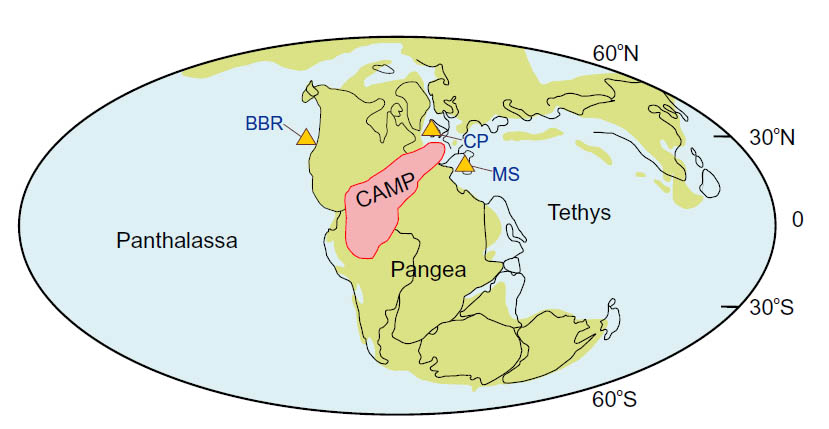
Pangaea just before the start of Atlantic opening at the end of the Triassic, showing the estimated extend of the CAMP large igneous province. The pink triangles show the sites investigated by He and colleagues.

At 201.3 Ma ago around 34 % of marine genera disappeared, comparable with the effect of the K-Pg extinction that ended the Mesozoic Era. Extinction of Triassic terrestrial animals is less quantifiable. Early dinosaurs made it through to diversify hugely during the succeeding Jurassic and Cretaceous Periods. Probably because nothing famous ceased to be or made its first appearance, the Tr-J mass extinction hasn’t captured public attention in the same way as those with the K-Pg or the P-Tr acronyms.  But it did dramatically alter the course of biological evolution. The extinctions coincided with a major eruption of flood basalts known as the Central Atlantic Magmatic Province (CAMP), whose relics occur on either side of the eponymous ocean, which began to open definitively at about the same time. So, chances are, volcanic emissions are implicated in the extinction event, somehow (see: Is end-Triassic mass extinction linked to CAMP flood basalts? June 2013). Tianchen He  of Leeds University, UK and the China University of Geosciences and British and Italian colleagues have studied three Tr-J marine sections on either side of Pangaea: in Sicily, Northern Ireland and British Columbia (He, T. and 12 others 2020. An enormous sulfur isotope excursion indicates marine anoxia during the end-Triassic mass extinction. Science Advances, v. 6, article eabb6704; DOI: 10.1126/sciadv.abb6704). Their objective was to test the hypothesis that CAMP resulted in an episode of oceanic anoxia that caused the many submarine organisms to become extinct. Since eukaryote life depends on oxygen, a deficit would put marine animals of the time under great stress. Such events in the later Mesozoic account for global occurrences of hydrocarbon-rich, black marine shales – petroleum source rocks – in which hypoxia thwarted complete decay of dead organisms over long periods. However there is scant evidence for such rocks having formed ~201 Ma ago. Such as there is dates to about 150 ka younger than the Tr-J boundary in an Italian shallow marine basin. The issue of evidence is compounded by the fact that there are no ocean-floor sediments as old as that, thanks to their complete subduction as Pangaea broke apart in later times and its continental fragments drifted to their present configuration.

But there is an indirect way of detecting deep-ocean anoxia, in the inevitable absence of any Triassic and early Jurassic oceanic crust. It emerges from what happens to the stable isotopes of sulfur when there are abundant bacteria that use the reduction of sulfate (SO42-) to sulfide (S2-) ions. Such microorganisms thrive in anoxic conditions and produce abundant hydrogen sulfide, which in turn leads to the precipitation of dissolved iron as minute grains of pyrite (FeS2). This biogenic process selectively excludes 34S from the precipitated pyrite. As a result, at times of widespread marine reducing conditions seawater as a whole becomes enriched in 34S relative to sulfur’s other isotopes. The enrichment is actually expressed in the unreacted sulfate ions, and they may be precipitated as calcium sulfate or gypsum (CaSO4) in marine sediments deposited anywhere: He et al. focussed on such fractionation. They discovered large ‘spikes’ in the relative enrichment of 34S at the Tr-J boundary in shallow-marine sedimentary sequences exposed at the three sites. Moreover, they were able to estimate that the conditions on the now vanished bed of the Triassic ocean that gave rise to the spikes lasted for about 50 thousand years. The lack of dissolved oxygen resulted in a five-fold increase in pyrite burial in the now subducted ocean-floor sediments of that time. The authors suggest that the oxygen depletion stemmed from extreme global warming, which, in turn, encouraged methane production by other ocean-floor bacteria and, in a roundabout way, other chemical reactions that consumed free dissolved oxygen. Quite a saga of a network of interactions in the whole Earth system that may hold a dreadful warning for the modern Earth and ourselves.

Centenary of the Milanković Theory

A letter in the latest issue of Nature Geoscience (Cvijanovic, I. et al. 2020. One hundred years of Milanković cycles, v. Nature Geoscience , v.13p. 524–525; DOI: 10.1038/s41561-020-0621-2) reveals the background to Milutin Milanković’s celebrated work on the astronomical  driver of climate cyclicity. Although a citizen of Serbia, he had been born at Dalj, a Serbian enclave, in what was Austro-Hungary. Just before the outbreak of World War I in 2014, he returned to his native village to honeymoon with his new bride. The assassination (29 June 2014) in Sarajevo of Archduke Franz Ferdinand by Bosnian-Serb nationalist Gavrilo Princip prompted Austro-Hungarian authorities to imprison Serbian nationals. Milanković was interned in a PoW camp. Fortunately, his wife and and a former Hungarian colleague managed to negotiate his release, on condition that he served his captivity, with a right to work but under police surveillance, in Budapest. It was under these testing conditions that he wrote his seminal Mathematical Theory of Heat Phenomena Produced by Solar Radiation; finished in 1917 but remaining unpublished until 1920 because of a shortage of paper during the war.

Curiously, Milanković was a graduate in civil engineering — parallels here with Alfred Wegener of Pangaea fame, who was a meteorologist — and practised in Austria. Appointed to a professorship in Belgrade in 1909, he had to choose a field of research. To insulate himself from the rampant scientific competitiveness of that era, he chose a blend of mathematics and astronomy to address climate change. During his period as a political prisoner Milanković became the first to explain how the full set of cyclic variations in Earth’s orbit — eccentricity, obliquity and precession — caused distinct variations in incoming solar radiation at different latitudes and changed on multi-thousand-year timescales. The gist  of what might have lain behind the cyclicity of ice ages had first been proposed by Scottish scientist James Croll almost half a century earlier, but it was Milutin Milanković who, as it were, put the icing on the cake. What is properly known as the Milanković-Croll Theory triumphed in the late 1970s as the equivalent of plate tectonics in palaeoclimatology after Nicholas Shackleton and colleagues teased out the predicted astronomical signals from time series of oxygen isotope variations in marine-sediment cores.

Appropriately, while Milanković’s revoluitionary ideas lacked corroborating geological evidence, one of the first to spring to his support was that other resilient scientific ‘prophet’, Alfred Wegener. Neither of them lived to witness their vindication.

The Younger Dryas and volcanic eruptions

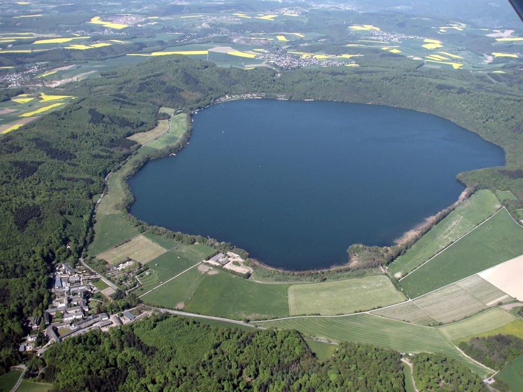
The issue of the Younger Dryas (YD) cold ‘hiccup’  between 12.9 to 11.7 thousand years (ka) ago during deglaciation and general warming has been the subject of at least 10 Earth-logs commentaries in the last 15 years (you can check them via the Palaeoclimatology logs). I make no apologies for what might seem to be verging on a personal obsession, because it isn’t. That 1200-year episode is bound up with major human migrations on all the northern continents: it may be more accurate to say ‘retreats’. Cooling to near-glacial climates was astonishingly rapid, on the order of a few decades at most. The YD was a shock, and without it the major human transition from foraging to agriculture might, arguably, have happened more than a millennium before it did. There is ample evidence that at 12.9 ka ocean water in the North Atlantic was freshened by a substantial input of meltwater from the decaying ice sheet on northern North America, which shut down the Gulf Stream (see: Tracking ocean circulation during the last glacial period, April 2005; The Younger Dryas and the Flood, June 2006). Such an event has many supporters. Less popular is that it was caused by some kind of extraterrestrial impact, based on various lines of evidence assembled by what amounts to a single consortium of enthusiasts. Even more ‘outlandish’ is a hypothesis that it all kicked off with radiation from a coincident supernova in the constellation Vela in the Southern sky, which is alleged to have resulted in cosmogenic 14C and 10Be anomalies at 12.9 ka. Another coincidence has been revealed by 12.9 ka-old volcanic ash in a sediment core from a circular volcanogenic lake or maar in Germany (see: Did the Younger Dryas start and end at the same times across Europe? January 2014). Being in a paper that sought to chart climate variations during the YD in a precisely calibrated and continuous core, the implications of that coincidence have not been explored fully, until now.

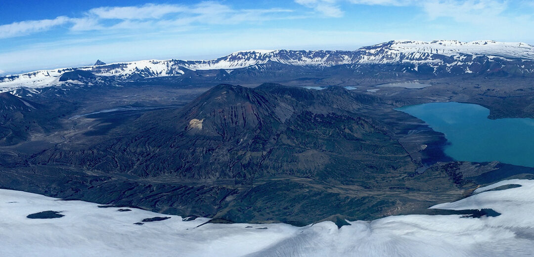
The Laacher See caldera lake in the recently active Eifel volcanic province in western Germany

A consortium of geochemists from three universities in Texas, USA has worked for some time on cave-floor sediments in Hall’s Cave, Texas as they span the YD. In particular, they sought an independent test of evidence for the highly publicised and controversial causal impact in the form of anomalous concentrations of the highly siderophile elements (HSE) osmium, iridium, platinum, palladium and rhenium (Sun, N. et al. 2020. Volcanic origin for Younger Dryas geochemical anomalies ca. 12,900 cal B.P.. Science Advances, v. 6, article eaax8587; DOI: 10.1126/sciadv.aax8587). There is a small HSE ‘spike’ at the 12.9 ka level, but there are three larger ones that precede it and one at about 11 ka. Two isotopes of the element osmium are often used to check the ultimate source of that element through the 187Os/188Os ratio, as can the relative proportions of the HSE elements compared with those in chondritic meteorites. The presence of spikes other than at the base of the YD does not disprove the extraterrestrial causal hypothesis, but the nature of those that bracket the mini-glacial time span not only casts doubt on it, they suggest a more plausible alternative. The 187Os/188Os data from each spike are ambiguous: they could either have arisen from partial melting of the mantle or from an extraterrestrial impact. But the relative HSE proportions point unerringly to the enriched layers having been inherited from volcanic gas aerosols. Two fit dated major eruptions of  the active volcanoes Mount Saint Helens (13.75 to 13.45 ka) and Glacier Peak (13.71 to 13.41 ka) in the Cascades province of western North America. Two others in the Aleutian and Kuril Arcs are also likely sources. The spike at the base of the YD exactly matches the catastrophic volcanic blast that excavated the Laacher See caldera in the Eifel region of western Germany, which ejected 6.3 km3 of sulfur-rich magma (containing 2 to 150 Mt of sulfur). Volcanic aerosols blasted into the stratosphere then may have dispersed throughout the Northern Hemisphere: a plausible mechanism for climatic cooling.

Sun et al. have not established the Laacher See explosion as the sole cause of the Younger Dryas. However, its coincidence with the shutdown of the Gulf Stream would have added a sudden cooling that may have amplified climatic effects of the disappearance of the North Atlantic’s main source of warm surface water. Effects of the Laacher See explosion may have been a tipping point, but it was one of several potential volcanic injections of highly reflective sulfate aerosols that closely precede and span the YD.

See also: Cooling of Earth caused by eruptions, not meteors (Science Daily, 31 July 2020)

Kicking-off planetary Snowball conditions

Untitled-1
Artist’s impression of the glacial maximum of a Snowball Earth event (Source: NASA)

Twice in the Cryogenian Period of the Neoproterozoic, glacial- and sea ice extended from both poles to the Equator, giving ‘Snowball Earth’ conditions. Notable glacial climates in the Phanerozoic – Ordovician, Carboniferous-Permian and Pleistocene – were long-lived but restricted to areas around the poles, so do not qualify as Snowball Earth conditions. It is possible, but less certain, that Snowball Earth conditions also prevailed during the Palaeoproterozoic at around 2.4 to 2.1 billion years ago. This earlier episode roughly coincided with the ‘Great Oxidation Event’, and one explanation for it is that the rise of atmospheric oxygen removed methane, a more powerful greenhouse gas than carbon dioxide, by oxidizing it to CO2 and water. That may well have been a consequence of the evolution of the cyanobacteria, their photosynthesis releasing oxygen to the atmosphere. The Neoproterozoic ‘big freezes’ are associated with rapid changes in the biosphere, most importantly with the rise of metazoan life in the form of the Ediacaran fauna, the precursor to the explosion in animal diversity during the Cambrian. Indeed all major global coolings, restricted as well as global, find echoes in the course of biological evolution. Another interwoven factor is the rock cycle, particularly volcanism and the varying pace of chemical weathering. The first releases CO2 from the mantle, the second helps draw it down from the atmosphere when weak carbonic acid in rainwater rots silicate minerals (see: Can rock weathering halt global warming, July 2020). All such interplays between major and sometimes minor ‘actors’ in the Earth system influence climate and, in turn, climate inevitably affects all the rest. With such complexity it is hardly surprising that there is a plethora of theories about past climate shifts.

As well as a link with fluctuations in the greenhouse effect, climate is influenced by changes in the amount of solar heating, for which there are yet more options to consider. For instance, the increase in Earth’s albedo (reflectivity) that results from ice cover, may lead through a feedback effect to runaway cooling, particularly once ice extends beyond the poorly illuminated poles. Volcanic dust and sulfate aerosols in the stratosphere also increase albedo and the tendency to cooling, as would interplanetary dust. More complexity to befuddle would-be modellers of ancient climates. Yet it is safe to say that, within the maelstrom of contributory factors, the freeze-overs of Snowball conditions must have resulted from our planet passing through some kind of threshold in the Earth System. Two theoretical scientists from the Department of Earth, Atmospheric, and Planetary Sciences at the Massachusetts Institute of Technology have attempted to cut through the log-jam by modelling the dynamics of the interplay between the ice-albedo feedback and the carbon-silicate cycle of weathering (Arnscheidt, C.W. & Rothman, D.H. 2020. Routes to global glaciation. Proceedings of the Royal Society A, v. 476, article 0303 online; DOI: 10.1098/rspa.2020.0303). Their mathematical approach involves two relatively simple, if long-winded, equations based on parameters that express solar heating, albedo, surface temperature and pressure, and the rate of volcanic outgassing of CO2; a simplification that sets biological processes to one side.

Unlike previous models, theirs can simulate varying rates, particularly of changes in solar energy input. The key conclusion of the paper is that if solar heating decreases faster than a threshold rate the more a planet’s surface water is likely to freeze from pole to pole. The authors suggest that a Snowball Earth event would result from a 2% fall in received solar radiation over about ten thousand years: pretty quick in a geological sense. Such a trigger might stem from a volcanic ‘winter’ scenario, an increase in clouds seeded by spores of primitive marine algae or other factors. The real ‘tipping point’ would probably be the high albedo of ice. There is a warning in this for the present, when a variety of means of decreasing solar input have been proposed as a ‘solution’ to global warming.

Because the Earth orbits the Sun in the ‘Goldilocks Zone’ and is volcanically active even global glaciation would be temporary, albeit of the order of millions of years. The cold would have shut down weathering so that volcanic CO2 could slowly build up in the atmosphere: the greenhouse effect would rescue the planet. Further from the Sun, a planet would not have that escape route, regardless of its atmospheric concentration of greenhouse gases: a neat lead-in to another recent paper about the ancient climate of Mars (Grau Galofre, A. et al. 2020. Valley formation on early Mars by subglacial and fluvial erosion. Nature Geoscience, early online article; DOI: 10.1038/s41561-020-0618-x)

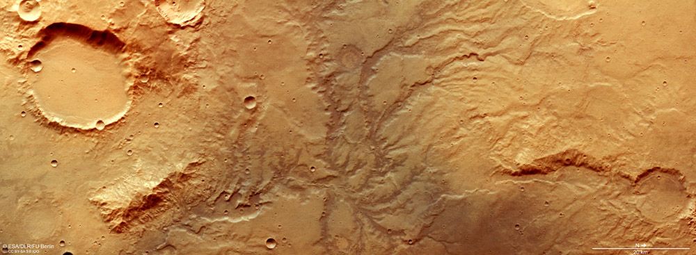
A Martian channel system: note later cratering (credit: European Space Agency)

There is a lot of evidence from both high-resolution orbital images of the Martian surface and surface ‘rovers’ that surface water was abundant over a long period in Mars’s early history. The most convincing are networks of channels, mainly in the southern hemisphere highlands. They are not the vast channelled scablands, such as those associated with Valles Marineris, which probably resulted from stupendous outburst floods connected to catastrophic melting of subsurface ice by some means. There are hundreds of channel networks, that resemble counterparts on Earth. Since rainfall and melting of ice and snow have carved most terrestrial channel networks, traditionally those on Mars have been attributed to similar processes during an early warm and wet phase. The warm-early Mars hypothesis extends even to interpreting the smooth low-lying plains of its northern hemisphere – about a third of Mars’s surface area – as the site of an ocean in those ancient times. Of course, a big question is, ‘Where did all that water go?’ Another relates to the fact that the early Sun emitted considerably less radiation 4.5 billion years ago than it does now: a warm-wet early Mars is counterintuitive.

Anna Grau Galofre of the University of British Columbia and co-authors found that many of the networks on Mars clearly differ in morphology from one another, even in small areas of its surface. Drainage networks on Earth conform to far fewer morphological types. By comparing the variability on Mars with channel-network shapes on Earth, the authors found a close match for many with those that formed beneath the ice sheet that covered high latitudes of North America during the last glaciation. Some match drainage patterns typical of surface-water erosion, but both types are present in low Martian latitudes: a suggestion of ‘Snowball Mars’ conditions? The authors reached their conclusions by analysing six mathematical measures that describe channel morphology for over ten thousand individual valley systems. Previous analyses of individual systems discovered on high-resolution images have qualitative comparisons with terrestrial geomorphology

See also: Chu, J. 2020. “Snowball Earths” May Have Been Triggered by a Plunge in Incoming Sunlight – “Be Wary of Speed” (SciTech Daily 29 July 2020); Early Mars was covered in ice sheets, not flowing rivers, researchers say (Science Daily, 3 August 2020)

Can rock weathering halt global warming?

The Lockdown has hardly been a subject for celebration, but there have been two aspects that are, to some extent, a comfort: the trickle of road traffic and the absence of convection trails. As a result the air is less polluted and much clearer, and the quietness, even in cities, has been almost palpable. Wildlife seems to have benefitted and far less CO2 has been emitted. Apart from the universal tension of waiting for one of a host of potential Covid-19 symptoms to strike and the fact that the world economy is on the brink of the greatest collapse in a century, it is tempting to hope that somehow business-as-usual will remain this way. B*gger the gabardine rush to work and the Great Annual Exodus to ‘abroad’. The crisis in the fossil fuel industry can continue, as far as I am concerned, But then, of course, I am retired, lucky to have a decent pension and live rurally. Despite the health risks, however, global capital demands that business-as-it-was must return now. A planet left to that hegemonic force has little hope of staving off anthropogenic ecological decline. But is there a way for capital to ‘have its cake and eat it’? Some would argue that there are indeed technological fixes. Among them is sweeping excess of the main greenhouse gas ‘under the carpet’ by burying it. There are three main suggestions: physically extracting CO2 where it is emitted and pumping it underground into porous rocks; using engineered biological processes in the oceans to take carbon into planktonic carbohydrate or carbonate shells and disposing the dead remains in soil or ocean-floor sediments; enhancing and exploiting the natural weathering of rock. The last is the subject of a recent cost-benefit analysis (Beerling, D.J. and 20 others 2020. Potential for large-scale CO2 removal via enhanced rock weathering with croplands. Nature, v. 583, p. 242–248; DOI: 10.1038/s41586-020-2448-9).

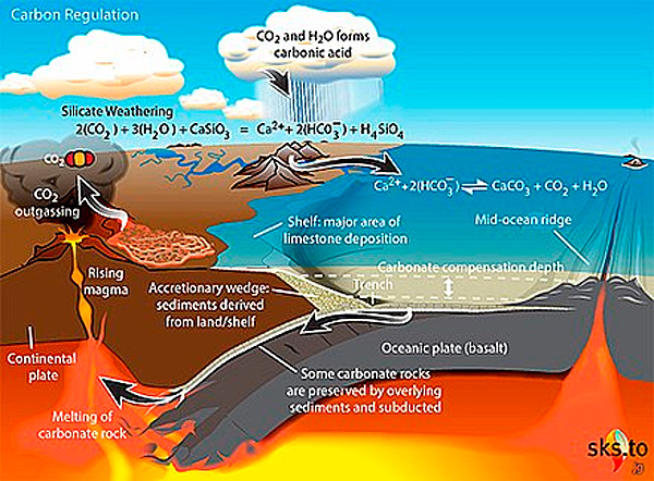
Carbon dioxide in the rock cycle (Credit: Skeptical Science, in Wikipedia)

Research into the climatic effects of rock weathering has a long history, for it represents one of the major components of the global carbon cycle, as well as the rock cycle. Natural chemical weathering is estimated to remove about a billion metric tons of atmospheric carbon annually. That is because the main agent of weathering is the slightly acid nature of rainwater, which contains dissolved CO2 in the form of carbonic acid (H2CO3). This weak acid comprises hydrogen ions (H+), which confer acidity, that are released by the dissolution of CO2 in water, together with HCO3ions (bicarbonate, now termed hydrogen carbonate). During weathering the hydrogen ions break down minerals in rock. This liberates metals that are abundant in the silicate minerals that make up igneous rocks – predominantly Na, Ca, K, and Mg – as their dissolved ions, leaving hydrated aluminium silicates (clay minerals) and iron oxides as the main residues, which are the inorganic basis of soils. The dissolved metals and bicarbonate ions may ultimately reach the oceans. However, calcium and magnesium ions in soil moisture readily combine with bicarbonate ions to precipitate carbonate minerals in the soil itself, a process that locks-in atmospheric carbon. Another important consequence of such sequestration is that it may make the important plant nutrient magnesium – at the heart of chlorophyll – more easily available and it neutralises any soil acidity built-up by continuous agriculture.  But carbon sequestration naturally achieved by weathering amounts to only about a thirtieth of that emitted by the burning of fossil fuels, and we know that is incapable of coping with the build-up of anthropogenic CO2 in the atmosphere: it certainly has not since the start of the Industrial Revolution.

What could chemical weathering do if it was deliberately enhanced?  One of the most common rocks, basalt, is made up of calcium-rich feldspar and magnesium-rich pyroxene and olivine. In finely granulated form this mix is particularly prone to weathering, and the magnesium released would enrich existing soil as well as drawing down CO2. Hence the focus by David Beerling and his British, US and Belgian colleagues on systematic spreading of ground-up basalt on cropland soils, in much the same way as crushed limestone is currently applied to reverse soil acidification. It is almost as cheap as conventional liming, with the additional benefit of fertilising: it would boost to crop yields. The authors estimate that removal of a metric ton of CO2 from the atmosphere by this means would cost between US$ 55 to 190, depending on where it was done. One of their findings is that the three largest emitters of carbon dioxide – China, the US and India – happen to have the greatest potential for carbon sequestration by enhanced weathering. Incidentally, increased fertility also yields more organic waste that itself could be used to increase the actual carbon content of soils, if converted through pyrolysis to ‘biochar’ .

It all sounds promising, almost ‘too good to be true’. The logistics that would be needed and the carbon emissions that the sheer mass of rock to be finely ground and then distributed would entail, for as long as global capital continues to burn fossil fuels, are substantial, as the authors admit. The grinding would have to be far more extreme than the production of igneous-rock road aggregate. Basalt or related rock is commonly used for resurfacing motorways, not especially well known for degrading quickly to a clay-rich mush. It would probably have to be around the grain size achieved by milling to liberate ore minerals in metal mines, or to produce the feedstock for cement manufacture: small particles create a greater surface area for chemical reactions. But there remains the issue of how long this augmented weathering would take to do the job: its efficiency. Experimental weathering to test this great-escape hypothesis is being conducted by a former colleague of mine, using dust from an Irish basalt quarry to coat experimental plots of a variety of soil types. After two months Mg and Ca ions were indeed being released from the dust, and tiny fragments of olivine, feldspar and pyroxene do show signs of dissolution. Whether this stems from rainwater – the main objective – or from organic acids and bacteria in the soils is yet to be determined. No doubt NASA is doing much the same to see if dusts that coat much of Mars can be converted into soils  Beerling et al. acknowledge that the speed of weathering is a major uncertainty. Large-scale field trials seem some way off, and are likely to be plagued by cussedness! Will farmers willingly change their practices so dramatically?

See also: Lehmann, J & Possinger, A. 2020. Removal of atmospheric CO2 by rock weathering holds promise for mitigating climate change. Nature, v. 583, p. 204-205; DOI: 10.1038/d41586-020-01965-7

Note (added 15 July 2020): Follower Walter Pohl has alerted me to an interesting paper on using ultramafic rocks in the same way (Kelemen, P.B. et al. 2020. Engineered carbon mineralization in ultramafic rocks for COremoval from air: Review and new insights. Chemical Geology, v.  550, Article 119628; DOI:10.1016/j.chemgeo.2020.119628). Walter’s own blog contains comments on the climatic efficacy of MgCO3 (magnesite) formed when olivine is weathered.

Turmoil in Roman Republic followed Alaskan volcanic eruption

That activities in the global political-economic system are now dramatically forcing change in natural systems is clear to all but the most obdurate. In turn, those changes increase the likelihood of a negative rebound on humanity from the natural world. In the first case, data from ice cores suggests that an anthropogenic influence on climate may have started with the spread of farming in Neolithic times. Metal pollution of soils had an even earlier start, first locally in Neanderthal hearths whose remains meet the present-day standards for contaminated soil, and more extensively once Bronze Age smelting of copper began. Global spread of anomalously high metal concentrations in atmospheric dusts shows up as ‘spikes’ in lead within Greenland ice cores during the period from 1100 BCE to 800 CE. This would have resulted mainly from ‘booms and busts’ in silver extraction from lead ores and the smelting of lead itself. In turn, that may reflect vagaries in the world economy of those times

Precise dating by counting annual ice layers reveals connections of Pb peaks and troughs with major historic events, beginning with the spread of Phoenician mining and then by Carthaginians and Romans, especially in the Iberian Peninsula. Lead reaches a sustained peak during the acme of the Roman Republic from 400 to 125 BC to collapse during widespread internal conflict during the Crisis of the Republic. That was resolved by the accession of Octavian/Augustus as Emperor in 31 BCE and his establishment of Pax Romana across an expanded empire. Lead levels rose to the highest of Classical Antiquity during the 1st and early 2nd centuries CE. Collapse following the devastating Antonine smallpox pandemic (165 to 193 CE) saw the ice-core records’ reflecting stagnation of coinage activity at low levels for some 400 years, during which the Empire contracted and changed focus from Rome to Constantinople. Only during the Early Medieval period did levels rise slowly to the previous peak.

The Okmok caldera on the Aleutian island of Umnak (Credit: Desert Research Institute, Reno, Nevada USA)

Earth-logs has previously summarised how natural events, mainly volcanic eruptions, had a profound influence in prehistory. The gigantic eruption of Toba in Sumatra (~73 ka ago) may have had a major influence on modern-humans migrating from Africa to Eurasia. The beginning of the end for Roman hegemony in the Eastern Mediterranean was the Plague of Justinian (541–549 CE), during which between 25 to 50 million people died of bubonic plague across the Eastern Empire. This dreadful event followed the onset of famine from Ireland to China, which was preceded by signs of climatic cooling from tree-ring records, and also with a peak of volcanogenic sulfate ions in the Greenland and Antarctic ice caps around 534 CE. Regional weakening of the populace by cold winters and food shortages, also preceded the Black Death of the mid-14th century. In the case of the Plague of Justinian, it seems massive volcanism resulted in global cooling over a protracted period, although the actual volcanoes have yet to be tracked down. Cooling marked the start of a century of further economic turmoil reflected by lead levels in ice cores (see above). Its historical context is the Early Medieval equivalent of world war between the Eastern Roman Empire, the Sassanid Empire of Persia and, eventually, the dramatic appearance on the scene of Islam and the Arabian, Syrian and Iraqi forces that it inspired (see: Holland, T. 2013. In the Shadow of the Sword: The battle for Global Empire and the End of the Ancient World. Abacus, London)

An equally instructive case of massive volcanism underlying social, political and economic turmoil has emerged from the geochemical records in five Greenlandic ice cores and one from the Siberian island of Severnaya Zemlya (McConnell, J.R. and 19 others 2020. Extreme climate after massive eruption of Alaska’s Okmok volcano in 43 BCE and effects on the late Roman Republic and Ptolemaic Kingdom. Proceedings of the National Academy of Sciences, recent article (22 June 2020); DOI: 10.1073/pnas.2002722117). In this case the focus was on ice layers in all six cores that contain sulfate spikes and, more importantly, abundant volcanic dust, specifically shards of igneous glass. Using layer counting, all six show major volcanism in the years 45 to 43 BCE. The Ides (15th) of March 44 BCE famously marked the assassination of Julius Caesar, two years after the Roman Republic’s Senate appointed him Dictator, following four years of civil war. This was in the later stages of the period of economic decline signified by the fall in ice-core levels of Pb (see above). The Roman commentator Servius reported “…after Caesar had been killed in the Senate on the day before, the sun’s light failed from the sixth hour until nightfall.” Other sources report similar daytime dimming, and unusually cold weather and famine in 43 and 42 BCE.

As well as pinning down the date and duration of the volcanic dust layers precisely (to the nearest month using laser scanning of the ice cores’ opacity), Joseph McConnell and the team members from the US, UK, Switzerland, Germany and Denmark also chemically analysed the minute glass shards from one of the Greenlandic ice cores. This has enabled them to identify a single volcano from 6 possible candidates for the eruption responsible for the cold snap: Okmok, an active, 8 km wide caldera in the Aleutian Islands of Alaska. Previous data suggest that its last major eruption was 2050 years ago and blasted out between 10 to 100 km3 of debris, including ash. Okmok is an appropriate candidate for a natural contributor to profound historic change in the Roman hegemony. The authors also use their ice-core data to model Okmok’s potential for climate change: it had a global reach in terms of temperature and precipitation anomalies. Historians may yet find further correlations of Okmok with events in other polities that kept annual records, such as China.

See also: Eruption of Alaska’s Okmok volcano linked to period of extreme cold in ancient Rome (Science Daily, 22 June 2020); Kornei, K. 2020. Ancient Rome was teetering. Then a volcano erupted 6,000 miles away. (New York Times, 22 June 2020)

Did an impact affect hunter gatherers at the start of the Younger Dryas?

Whether or not the return to a glacial climate between 12.8 and 11.7 thousand years (ka) ago, known as the Younger Dryas (YD), was triggered by some kind of extraterrestrial impact has been a hot and sometimes fractious issue since 2007 (see: Whizz-bang view of Younger Dryas; Earth-logs, July 2007). Before then the most favoured causal mechanism was a shutdown of the Gulf Stream’s Arctic warming influence as a result of some kind of catastrophic flooding of fresh water into the North Atlantic. That would have lowered the density of surface waters, thereby preventing them from sinking to drive the deep circulation that draws surface water from the tropics into high northern latitudes (see: The Younger Dryas flood; May 2010). In 2008 the melt-water flood supporters were sufficiently piqued by the suggestion of a hitherto unsuspected impact event to mount a powerful rejoinder (see: Impact cause for Younger Dryas draws flak; May 2008), casting doubt on the validity of the data that had been presented. It seemed like a repeat of the initial furore over claims for a ‘mountain falling out of the sky’ wiping out the dinosaurs and much else. Yet, like the claims by Alvarez pere et fils for the K-T impact, accumulated weight of evidence published by its protagonists eventually has given the idea of an impact trigger for the YD a measure of respectability. This began with evidence of an impact crater beneath the Greenland icecap (see: Subglacial impact structure in Greenland: trigger for Younger Dryas?; November 2018), then signs of a 12.8 ka fire storm in Chile followed by geochemical evidence from South Carolina, USA for a coinciding impact (see: More on the Younger Dryas causal mechanism; November 2019).

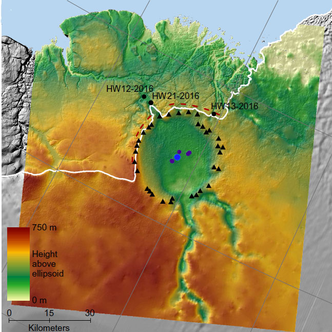
Colour-coded subglacial topography from radar sounding over the Hiawatha Glacier of NW Greenland, showing a possible impact crater (Credit: Kjaer et al. 2018; Fig. 1D)

The YD played havoc with humans who had begun to repopulate northern Europe from their Ice Age refuges in the south and those who had first ventured into the Americas  across the Beringia land bridge between Siberia and Alaska. The climate decline was extremely rapid, spanning a mere decade or so, and many would have been trapped to perish in what again became frigid steppe land. There is now evidence that late-Palaeolithic to Mesolithic hunter gatherers living far south of the reglaciated zone also suffered devastation at the start of the YD (Moore, A.M.T. and 13 others 2020. Evidence of Cosmic Impact at Abu Hureyra, Syria at the Younger Dryas Onset (~12.8 ka): High-temperature melting at > 2,200 °C. Nature Science Reports, v. 10, p. 1-22; doi: 10.1038/s41598-020-60867-w). Abu Hureyra is a tell – a mound settlement – originally on the banks of the Euphrates in northern Syria. It now lies beneath Lake Assad, but was excavated in the early 1970s to reveal a charcoal-littered habitation surface with signs of a settlement and some cultivation. Charcoal from archived samples yielded a precise radiocarbon age of 12825 ± 55 ka, coinciding with the start of the YD. The sediment from the habitation floor also contained signs compatible with ejecta from a high-energy impact: tiny diamonds and glass spherules. Analyses of the glass by the authors suggests that it formed at a temperature up to 2200°C, far greater than that of magma associated with a volcanic eruption or in hearths used by the inhabitants. However, others have analysed the glass and suggest more mundane temperatures that could be explained more simply by accidental burning of thatched huts. That possibility might explain the lack of other impact indicators, such as shocked mineral grains and anomalous geochemistry, particularly the platinum-group metals that were the original ‘smoking gun’ for the K-T boundary event and other major impacts. Incidentally, these crucial indicators have been reported from other YD sites investigated by several members of the team behind this paper. My view is that what seems to be a remarkable coincidence will not settle the matter, but will probably draw the same kind of ‘flak’ as did others on this topic. It is hardly likely that new samples will be collected from the now submerged Abu Hureyra site.

See also: Cometary Debris may have destroyed Paleolithic settlement 12,800 years ago (Science News. 2 July 2020)

Update on climate and sea-level change during the Cenozoic

The Cenozoic Era was a period of fundamental change in the outer part of the Earth system. It culminated in the greatest climatic cooling since the Permian Period, during which upright apes emerged between 6 to 10 Ma ago.  The most decisive part of hominin evolution – the appearance of our own genus Homo – took place in the last 2.5 Ma that saw icecaps plastered over both polar regions and repeated pulses of major climate upheaval that dramatically affected all parts of the continents. Whereas the Mesozoic was dominated by reptiles, most famously the dinosaurs, the Cenozoic is rightly known as the age of mammals and of birds. The flowering plants, especially grasses, also transformed terrestrial ecosystems. The background to what has become ‘our time’ is not only climate change, but massive shifts in sea level and the outlines of the continents. For more than two decades many palaeoclimatologists have focused on the Cenozoic, gathering data using a variety of rapidly advancing technologies from a growing number of sites, in sediments from the continents and the ocean floor. One problem has been correlating all this global data precisely, coming as it does from many incomplete sedimentary sequences dotted around the planet. A great deal of basic information has come from the petroleum industry, which, of course, has continually eyed sedimentary rocks as the source of hydrocarbons through the 20th century. It was seismic reflection surveying that first gave clues to global ups and downs of sea level from onlaps and offlaps of strata that are visible on seismic sections, amplified by sequence stratigraphy. Six geoscientists from Rutgers University in New Jersey, USA have blended oil-industry archives with academic research to produce the first fully calibrated, comprehensive record of the Cenozoic (Miller, K.G. et al. 2020. Cenozoic sea-level and cryospheric evolution from deep-sea geochemical and continental margin records. Science Advances, v. 6, article eaaz1346; DOI: 10.1126/sciadv.aaz1346).

Latest palaeoclimate data for the Cenozoic Era. A oxygen-isotope data from benthic foraminifera (pale blue = polar icecaps, green = ice-free, pink – hothouse); B estimated mean sea-surface temperature from the calcium/magnesium ratio in Pacific Ocean cores; C variation in global mean sea level estimated from A and corrected for changes in the density of seawater due to water temperature (B); D atmospheric CO2 variations estimated using various proxies – see top right box. Click on the image to show a full-size version in a new browser tab. (Credit: Miller et al. 2020; Fig. 1)

Fluctuations in the proportion of 18O (δ18O) in the tests of foraminifera that lived in deep water are the key to global changes in sea level  and point to the influence of glacial ice accumulating on land (see Cooling sets in: Stepping Stones, Chapter 17). This is because glaciers are made from water that has evaporated from the oceans. When this happens, water that incorporates the lighter 16O isotope evaporates more easily and becomes enriched in atmospheric water vapour. When this water falls as snow that accumulates on land to form ice, the oceans are slightly enriched in the heavier 18O: δ18O incorporated into the shelly material of organism dwelling in the deep ocean increases at levels of a few parts per thousand. Conversely, their δ18O decreases when huge ice caps melt (A on the figure). The oxygen isotope records from fossils in ocean floor sediments give a far more precise impression of fluctuating sea level than do seismic sections and sequence stratigraphy of sedimentary rocks that interest the oil industry. But it is an ‘impression’, because other factors affect sea level.

Not only the global volume of ocean water is involved: the volume of the ocean basins changes too. This can occur because of changes in the rate of sea-floor spreading: when that is fast the hot new oceanic lithosphere is less dense and so buoys-up part of the ocean floor to drive sea level upwards. Slow spreading does the converse, as more lithosphere cools and sinks slightly. Another factor is the changing rate of marine sedimentation of material eroded from the continents. That fills ocean basins to some extent, again displacing the water upwards. When sediments are compacted as they become more deeply buried that has an effect too, to increase basin volume and result in sea-level fall. Oil industry geoscientists have attempted to allow for these long-term, slow mechanisms, to give a more accurate sea-level record.

Yet there is another important factor: the density and thus volume of ocean water changes with temperature. The warmer it is the greater the volume of ocean water and the higher is sea level. This is where academic work comes in handy. Two common elements that are dissolved in ocean water are magnesium and calcium. They also occur in the carbonate tests of the same deep-water forams that are used for oxygen-isotope measurements. It turns out that the warmer the water is the more magnesium enters the foram tests, and vice versa: their Mg/Ca ratio is a reliable proxy for mean ocean temperature and can be measured easily, centimetre-by-centimetre through cores. Kenneth Miller and colleagues have used this with the oxygen isotope proxy for land-ice volume to correct the sea-level record.

The Cenozoic ocean temperature record (B on the figure) is, in itself, interesting. It reveals far more large fluctuations than previously thought, especially in the Palaeocene and early Eocene. Yet, overall, the trend is one of steady cooling compared with the sudden shifts in δ18O that mark the onset of the Antarctic ice cap at the Eocene-Oligocene boundary around 34 Ma ago, and the apparent, temporary emergence from ‘ice-house conditions in the Middle Miocene. Also, sea level corrected for ocean temperature effects (C on the figure) suggests that for much of the Cenozoic sea level was lower than expected; i.e. it rarely exceeded 60 m above the current level, which is that expected when no substantial mass of  land ice exists.

The other important compilation made by Miller et al. is that of the CO2 content of the atmosphere estimated using six different proxies. It is a lot more fuzzy than the oceanic records because the proxies are not precise. Nevertheless, it is interesting. The current, partly anthropogenic level of around 400 parts per million (ppm) is not unique. In fact from 55 to 23 Ma it was consistently above this ‘Anthropocene’ level, peaking at twice that level at the end of the Eocene. That’s odd, because it doesn’t tally with the oxygen isotopes that indicate the onset of large scale Antarctic glaciation shortly afterwards. In fact most of the climatic highlights shown by A on the figure are not reflected in the Cenozoic history of the most influential greenhouse gas. In the short term of glacial-interglacial cycles during the late Pleistocene, atmospheric CO2 levels are very closely related to fluctuations of land-ice volume. In the 65 Ma of the Cenozoic such a link is hard to argue for. There are more puzzles than revelations in this otherwise major addition to palaeoclimatology.

Alternative explanation for interglacial climate instabilities; and a warning

For the past two and a half million years there has been no such thing as a stable climate on our home world. The major fluctuations that have given rise to glacial and interglacial episodes and the times that separate them are most familiar, as is their connection with the periodicity of gravitational effects on the Earth’s orbital and rotational behaviour. There are mysteries, such as the dominance of a ~100 ka cyclicity with the least effect on solar heating since a million years ago and the shift that took place then from dominant ~40 ka cycles that preceded it. But over shorter time scales there are more irregular climatic perturbations that can not be attributed to gravity variations in the Inner Solar System. In the run-up to maximal glacial conditions in the Northern Hemisphere are changes in the isotopic records that reveal increases and decreases in the mass of ice on continental masses. Known as Dansgaard-Oeschger events they occurred on a (very) roughly 10 ka basis and lasted between 1000 and 2000 years. They resulted in rapid temperature changes spanning up to 15°C over the Greenland ice cap and have been explained by changes in surface- and deep-water circulation within the North Atlantic. Effectively, the Gulf Stream and the thermohaline circulation that drives it were periodically shut down and turned on. Even more irregular in occurrence are sudden global coolings in the midst of general warming into interglacial episodes. The most spectacular of these was the Younger Dryas cooling to almost full-glacial conditions between 12.8 and 11.5 ka, at a time when the Earth had achieved a mean surface temperature almost as high as that which has prevailed over the last 11,000 years.  There have been lesser cold ‘snaps’ during the Holocene, and in every one of the earlier interglacials for which there are data. Their occurrence seems unpredictable, even chaotic.

In 2006 the Younger Dryas was explained as the result of massive amounts of freshwater flooding into the Arctic Ocean from huge, ice-dammed lakes in North America. Decreased density of the high-latitude surface water resulted in its failure to sink and thus drive thermohaline circulation (see The Younger Dryas and the Flood June 2006). This hypothesis has subsequently been applied to other such sudden climatic events, such as the cooling episode around 8.2 ka during the Holocene. A recent study set out to test this notion from ocean-floor records of the last half-million years (Galaasen, E.V. and 9 others 2020. Interglacial instability of North Atlantic Deep Water ventilation. Science, v. 367, p. 1485-1489; DOI: 10.1126/science.aay6381). The data are from a seafloor sediment core in a trough south of Greenland, where cold, salty and dense bottom water flows southward from the Arctic to drag warmer surface water northwards in the Gulf Stream to replace it. That warm surface water has a high salinity because of evaporation in the tropics, so once it cools it sinks, thereby maintaining thermohaline circulation.

Modelled circulation rate of Atlantic circulation during 10 ka of the last interglacial before the Holocene (credit: Thomas Stocker, 2020 Science)

Eirik Galaasen of the University of Bergen and colleagues from several countries flanking the North Atlantic found large, abrupt changes in the mass flow of water through the trough – based on studies of carbon isotopes in bottom-living foraminifera – during each of the four interglacials that preceded the current one. The higher the δ13C in the forams the more vigorous the deep flow, whereas low values suggest weak flow or stagnation, due to waning of thermohaline circulation. Transition between the two states is rapid and each state lingered for several centuries. While the Holocene records only one such perturbation of note, that at 8.2 ka, previous interglacials reveal dozens of them. One possibility is that the thermohaline circulation system of the North Atlantic behaved in a chaotic fashion during previous interglacial episodes, producing similarly erratic shifts in climate. Seemingly, the Holocene bucks the trend, which may have added an element of luck to the establishment of human agricultural economies throughout that Epoch. All the signs are that current, anthropogenic global warming will slow down the water circulation in the North Atlantic. Might that set-off what seems to have been the norm of chaotic interglacial climate shifts for the best part of that half-million years? Hard to tell, without more studies …

See also: Stocker, T.F. 2020. Surprises for climate stability. Science, v. 367, p. 1425-1426; DOI: 10.1126/science.abb3569; How stable is deep ocean circulation in warmer climate? (Science Daily)

Soluble iron and global climate

The environment that humans inhabit is better described as the Earth System, for a good reason. Every part of our planet, the living and the seemingly inert, from the core to the outermost atmosphere, is and always has been interacting with all the others in one way or another. Earth-logs aims to express that, as does my recently revised and now free book Stepping Stones. The vagaries of the Earth’s climate present good examples, the most obvious being the role of chemistry in the form of atmospheric greenhouse gases, especially carbon dioxide, and their interaction with other parts of the Earth System.

Carbon and oxygen atoms that make up CO2 are also present in dissolved form in rain, freshwater and the oceans as the dissolved gas itself, carbonic acid (H2CO­3­) and the soluble bicarbonate ion HCO3, in proportions that depend on water temperature and acidity (pH). Those forms make the oceans an extremely large ‘sink’ for carbon; i.e. CO2 in dissolved form is removed from the atmospheric greenhouse effect. In the short term, there is a rough balance because water bodies also emit CO2, particularly when they heat up.

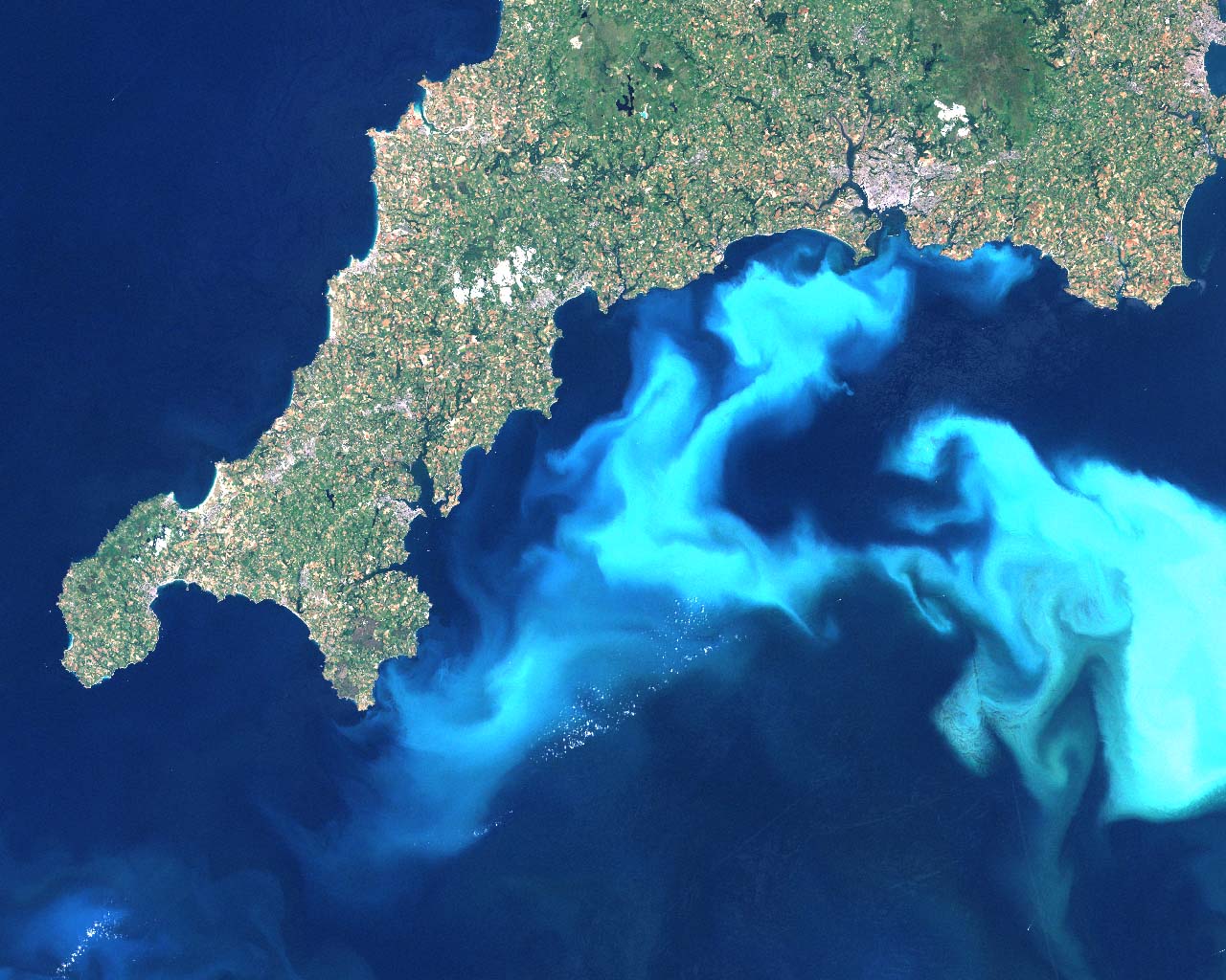
Phytoplankton bloom in the Channel off SW England (Landsat image)

Carbon dioxide enters more resilient forms through the marine part of the biosphere, at the base of which is photosynthesising phytoplankton. Photosynthesisers ‘sequester’ CO2 from the oceans as various carbohydrates in their soft tissue. Some of them use bicarbonate ions to form calcium carbonate in shells or tests. Once the organisms die both their soft and hard parts may end up buried in ocean-floor sediments: a longer-term sink. How much carbon is buried in these two forms depends on whether bacteria break down the soft tissues by oxidation and on the acidity of water that tends to dissolve the carbonate. Both processes ultimately yield dissolved CO2 that returns to the atmosphere.

Even the simplest phytoplankton cannot live on carbon dioxide and water alone: they need nutrients. The most familiar to any gardener are nitrogen, phosphorus and potassium. These are mainly supplied in runoff from the continents; although marine upwellings supply large amounts where deep ocean water is forced to the surface. Large tracts in the central parts of the oceans are, in effect, marine deserts whose biological productivity is very low. Surprisingly this is not because of severe shortages of N, P and K. This is because a key nutrient, albeit a minor one, is missing; dissolved iron that phytoplankton and ocean fertility in general depend on. This was discovered in the 1970s by US oceanographer John Martin. Just how important iron is to fertility of the oceans and to global climate emerged from studies of ice cores from the Antarctic ice sheet. Air bubbles in the myriad annual layers reveal that their CO2 content falls with each change in oxygen isotopes related to the periodic build up of polar ice caps during cold periods. The greenhouse effect diminished as a result during each stadial, for the simple reason that up to a third of all atmospheric carbon dioxide – about 200 billion tonnes – was withdrawn. The clearest of these are at the last glacial maximum and during the rapid build up glacial ice between 70 and 60 thousand years ago; a time of low sea level when a major ‘out-of-Africa’ human migration took place. A possible candidate for achieving this could have been massively increased ocean fertility and the burial of dead phytoplankton and their shells.

Analyses of Antarctic ice cores record fluctuations in atmospheric CO2 trapped in bubbles during the last ice age (top) and how iron-rich dust deposition onto the ice increased hugely during two major cold periods (bottom) – the last glacial maximum (35 to 18 ka) and between 70 and 60 ka. (Credit, Stoll; Fig. 1)

During stadials the ice cores also reveal that a great deal more dust found its way from the continents to the polar ice sheets. Analysing the dusty layers showed that to have included lots of iron. Falling into the cold ocean-surface waters around the polar regions would have added this crucial nutrient to a medium already rich in CO2 – the colder water is the more gas it will dissolve. These distant oceans bloomed with phytoplankton, speeding up the sequestration of carbon into ocean-floor sediments. Iron may have triggered a biological pump of gargantuan proportions that amplified ice-age cooling. Today the remotest parts of the world’s oceans are starved of iron so the pump only functions in a few places where iron is supplied by rivers or upwellings of deep ocean water

The marine biosphere is clearly a very important active component in the Earth’s climate subsystem. Climate’s continually changing interactions with the rest of the Earth System make climate change hugely complex. It is difficult to predict but growing understanding of its past behaviour is helpful. The late John Martin’s hypothesis of the effects on climate of changing iron concentrations in surface ocean water has a corollary: the stronger the biological pump the more oxygen in deep water must be used up in bacterial decay of descending organic matter. Indeed it was as recent estimates of the degree of oxygenation in ocean-sediment layers correlate with changes in climate that they also reveal.

So, would deliberate iron-fertilisation of polar oceans help draw down greenhouse warming? When several small patches of the Southern Ocean were injected with a few tonnes of dissolved iron they did indeed respond with phytoplankton blooms. However, it is impossible to tell if that had any effect on the atmosphere. ‘Going for broke’ with a massive fertilisation of this kind has been proposed, but this ventures dp into the political swamp that currently surrounds global warming and the wider environment. It is becoming possible to model such a strategy by using the data from the experiments and from ice cores, and early results seem to confirm the role of iron and the biological pump in CO2 sequestration by suggesting that half the known draw-down during ice ages can be explained in this way.

Based on a review by: Heather Stoll in February 2020. (30 years of the iron hypothesis of ice ages. Nature, v. 578, p. 370-371; DOI: 10.1038/d41586-020-00393-x}

Finding Archaean atmospheric composition using micrometeorites

Modern micrometeorites (about 20 μm in diameter) from deep-sea sediments, with shiny magnetite-rich veneers (Credit: D. E. Brownlee)

The gases making up the Earth’s atmosphere and their relative proportions before 2.5 billion years (Ga) ago are known with very little certainty. Carbonate rocks are rare, indicating that the oceans were more acidic, which implies that they had dissolved more CO2 from the atmosphere, which, in turn implies that there was much more of that gas than in present air. There are few signs of widespread glaciogenic sediments of Archaean age, at a time when the Sun’s energy output is estimated to have been at 70 to 75% of its present level. Without an enhanced greenhouse effect oceans would have been frozen over; so that supports high CO2 concentrations too. The fact that water worn grains of minerals such as uraninite (UO2) and pyrite (FeS2), which are stable only in reducing conditions, occur in Archaean conglomerates is a good indicator that there were only vanishingly small amounts of oxygen in the air. That was not to change until marine photosynthesisers produced enough to overcome the general reducing conditions at the Earth’s surface, marked by the Great Oxidation Event at around 2.4 Ga (see: Massive event in the Precambrian carbon cycle; Earth-logs, January 2012. Search for more articles in sidebar at Earth-logs home page). It was then that ancient soils (palaeosols) became the now familiar red colour because of their content of ferric iron oxides and hydroxides The problem is that reliable numbers cannot be attached to these kinds of observation. A common means of estimating CO2 levels comes from the way in which the gas reacts with silicates as soils form at the land surface, estimated from carbon isotopes in soil carbonate nodules. Since the rise of land plants around 400 Ma ago the distribution of pores (stomata) in fossil leaves provides a more precise estimate: the more CO2 in air the less densely packed are leaf stomata. For the Precambrian we are stuck with estimates based on chemical reactions of minerals with the atmosphere. Until recently, one reaction that must always have been extremely common was overlooked.

When meteorite pass through the atmosphere at very high speed friction heats them to incandescence. Their surfaces not only melt but the minerals from which they are composed react very strongly with air. The reaction products should therefore provide chemical clues to the relative proportions of atmospheric gases. Both oxygen and carbon dioxide are reactive at such temperatures, although nitrogen is virtually inert, yet it tends to buffer oxidation reactions. The rest of the atmosphere comprises noble gases – mainly argon – and by definition they are completely unreactive. Pure-iron micrometeorites collected from 2.7 Ga old sediments in the Pilbara Province of Western Australia are veneered with magnetite (Fe3O4) and wüstite (FeO), thus preserving a record of their passage through the Neoarchaean atmosphere. If the oxidant had been oxygen, for these minerals to form from elemental iron suggests oxygen levels around those prevailing today: clearly defying the abundant evidence for its near-absence during the Archaean. Carbon dioxide is the only candidate. Two studies have produced similar results (Lehmer, O. R. et al. 2020. Atmospheric CO2 levels from 2.7 billion years ago inferred from micrometeorite oxidationScience Advances, v. 6, article aay4644;  DOI: 10.1126/sciadv.aay4644 and Payne, R.C. et al. 2020. Oxidized micrometeorites suggest either high pCO2 or low pN2 during the Neoarchean. Proceedings of the National Academy of Sciences, v. 117 1360 DOI:10.1073/pnas.1910698117). Both use complex modelling of the chemical effects of meteorite entry. Lehmer and colleagues estimated that the Neoarchaean atmosphere contained about 64% CO2, with a surface atmospheric pressure about half that at present. This would be sufficient for a surface temperature of about 30°C achieved by the greenhouse effect, taking into account lower solar heating. The team led by Payne concluded a lower concentration (25 to 50%) and a somewhat cooler planet at that time. Both results suggest ocean water considerably more acid than are today’s. The combined warmth and acidity would have had a fundamental bearing on both the origin, survival and evolution of early life.

See also: Carroll, M. 2020. Meteorites reveal high carbon dioxide levels on early Earth; Yirka, R. Computer model shows ancient Earth with an atmosphere 70 percent carbon dioxide. (both from Phys.org)

Closure for the K-Pg extinction event?

Anyone who has followed the saga concerning the mass extinction at the end of the Cretaceous Period (~66 Ma ago) , which famously wiped out all dinosaurs except for the birds, will know that its cause has been debated fiercely over four decades. On the one hand is the Chicxulub asteroid impact event, on the other the few million years when the Deccan flood basalts of western India belched out gases that would have induced major environmental change across the planet. Support has swung one way or the other, some authorities reckon the extinction was set in motion by volcanism and then ‘polished-off’ by the impact, and a very few have appealed to entirely different mechanism lumped under ‘multiple causes’. One factor behind the continuing disputes is that at the time of the Chicxulub impact the Deccan Traps were merrily pouring out Disentanglement hangs on issues such as what actual processes directly caused the mass killing. Could it have been starvation as dust or fumes shut down photosynthesis at the base of the food chain? What about toxic gases and acidification of ocean water, or being seared by an expanding impact fireball and re-entering incandescent ejecta? Since various lines of evidence show that the late-Cretaceous atmosphere had more oxygen that today’s the last two may even have set the continents’ vegetation ablaze: there is evidence for soots in the thin sediments that mark the K-Pg boundary. The other unresolved issue is timing: of volcanogenic outgassing; of the impact, and of the extinction itself. A new multi-author, paper may settle the whole issue (Hull, P.M and 35 others 2020. On impact and volcanism across the Cretaceous-Paleogene boundary. Science, v. 367, p. 266-272; DOI: 10.1126/science.aay5055).

K-Pg oxygen
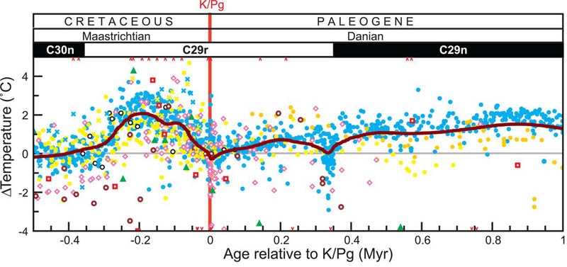
Marine temperature record derived from δ18O and Mg/Ca ratios spanning 1.5 Ma that includes the K-Pg boundary: the bold brown line shows the general trend derived from the data points (Credit: Hull et al. 2020; Fig 1)

The multinational team approached the issue first by using oxygen isotopes and the proportion of magnesium relative to calcium (Mg/Ca ratio) in fossil marine shells (foraminifera and molluscs) in several ocean-floor sediment cores, through a short interval spanning the last 500 thousand years of the Cretaceous and the first  million years of the Palaeocene. The first measures are proxies for seawater temperature. The results show that close to the end of the Cretaceous temperature rose to about 2°C above the average for the youngest Cretaceous (the Maastrichtian Age; 72 to 66 Ma) and then declined. By the time of the mass extinction (66 Ma) sea temperature was back at the average and then rose slightly in the first 200 ka of Palaeocene to fall back to the average at 350 ka and then rose slowly again.

Changes in carbon isotopes (δ13C) of bulk carbonate samples from the sediment cores (points) and in deep-water foraminifera (shaded areas) across the K-Pg boundary. (Credit: Hull et al. 2020; Fig 2A)

The second approach was to look in detail at carbon isotopes (δ13C) – a measure of changes in the marine carbon cycle –  and oxygen isotopes (δ18O) in deep water foraminifera and bulk carbonate from the sediment cores, in comparison to the duration of Deccan volcanism (66.3 to 65.4 Ma). The δ13C measure from bulk carbonate stays roughly constant in the Maastrichtian, then falls sharply at 66 Ma.  The δ13C of the deep water forams rises to a peak at 66 Ma. The δ18O measure of temperature peaks and declines at the same times as it does for the mixed fossils. Also examined was the percentage of coarse sediment grains in the muds from the cores. That measure is low during the Maastrichtian and then rises sharply at the K-Pg boundary.

Since warming seems almost certainly to be a reflection of CO2 from the Deccan (50 % of total Deccan outgassing), the data suggest not only a break in emissions at the time of the mass extinction but also that by then the marine carbon system was drawing-down its level in air. The δ13C data clearly indicate that the ocean was able to absorb massive amounts of CO2 at the very time of the Chicxulub impact and the K-Pg boundary. Flood-basalt eruption may have contributed to the biotic aftermath of the extinction for as much as half a million years. The collapse in the marine fossil record seems most likely to have been due to the effects of the Chicxulub impact. A third study – of the marine fossil record in the cores – undertaken by, presumably, part of the research team found no sign of increased extinction rates in the latest Cretaceous, but considerable changes to the marine ecosystem after the impact. It therefore seems that the K-Pg boundary impact ‘had an outsized effect on the marine carbon cycle’. End of story? As with earlier ‘breaks through’; we shall see.

See also: Morris, A. 2020 Earth was stressed before dinosaur extinction (Northwestern University)

How marine animal life survived (just) Snowball Earth events

diamict3
A Cryogenian glacial diamictite containing boulders of many different provenances from the Garvellach Islands off the west coast of Scotland. (Credit: Steve Drury)

Glacial conditions during the latter part of the Neoproterozoic Era extended to tropical latitudes, probably as far as the Equator, thereby giving rise to the concept of Snowball Earth events. They left evidence in the form of sedimentary strata known as diamictites, whose large range of particle size from clay to boulders has a range of environmental explanations, the most widely assumed being glacial conditions. Many of those from the Cryogenian Period are littered with dropstones that puncture bedding, which suggest that they were deposited from floating ice similar to that forming present-day Antarctic ice shelves or extensions of onshore glaciers. Oceans on which vast shelves of glacial ice floated would have posed major threats to marine life by cutting off photosynthesis and reducing the oxygen content of seawater. That marine life was severely set back is signalled by a series of perturbations in the carbon-isotope composition of seawater. Its relative proportion of 13C to 12C (δ13C) fell sharply during the two main Snowball events and at other times between 850 to 550 Ma. The Cryogenian was a time of repeated major stress to Precambrian life, which may well have speeded up evolution, sediments of the succeeding Ediacaran Period famously containing the first large, abundant and diverse eukaryote fossils.

For eukaryotes to survive each prolonged cryogenic stress required that oxygen was indeed present in the oceans. But evidence for oxygenated marine habitats during Snowball Earth events has been elusive since these global phenomena were discovered. Geoscientists from Australia, Canada, China and the US have applied novel geochemical approaches to occasional iron-rich strata within Cryogenian diamictite sequences from Namibia, Australia and the south-western US in an attempt to resolve the paradox (Lechte, M.A. and 8 others 2019. Subglacial meltwater supported aerobic marine habitats during Snowball Earth. Proceedings of the National Academy of Sciences, 2019; 201909165 DOI: 10.1073/pnas.1909165116). Iron isotopes in iron-rich minerals, specifically the proportion of 56Fe relative to that of 54Fe (δ56Fe), help to assess the redox conditions when they formed. This is backed up by cerium geochemistry and the manganese to iron ratio in ironstones.

In the geological settings that the researchers chose to study there are sedimentological features that reveal where ice shelves were in direct contact with the sea bed, i.e. where  they were ‘grounded’. Grounding is signified by a much greater proportion of large fragments in diamictites, many of which are striated through being dragged over underlying rock. Far beyond the grounding line diamictites tend to be mainly fine grained with only a few dropstones. The redox indicators show clear changes from the grounding lines through nearby environments to those of deep water beneath the ice. Each of them shows evidence of greater oxidation of seawater at the grounding line and a falling off further into deep water. The explanation given by the authors is fresh meltwater flowing through sub-glacial channels at the base of the grounded ice fed by melting at the glacier surface, as occurs today during summer on the Greenland ice cap and close to the edge of Antarctica. Since cold water is able to dissolve gas efficiently the sub-glacial channels were also transporting atmospheric oxygen to enrich the near shore sub-glacial environment of the sea bed. In iron-rich water this may have sustained bacterial chemo-autotrophic life to set up a fringing food chain that, together with oxygen, sustained eukaryotic heterotrophs. In such a case, photosynthesis would have been impossible, yet unnecessary. Moreover, bacteria that use the oxidation of dissolved iron as an energy source would have caused Fe-3 oxides to precipitate, thereby forming the ironstones on which the study centred. Interestingly, the hypothesis resembles the recently discovered ecosystems beneath Antarctic ice shelves.

Small and probably unconnected ecosystems of this kind would have been conducive to accelerated evolution among isolated eukaryote communities. That is a prerequisite for the sudden appearance of the rich Ediacaran faunas that colonised sea floors globally once the Cryogenian ended. Perhaps these ironstone-bearing diamictite occurrences where the biological action seems to have taken place might, one day, reveal evidence of the precursors to the largely bag-like Ediacaran animals

Risks of sudden changes linked to climate

The Earth system comprises a host of dynamic, interwoven components or subsystems. They involve processes deep within Earth’s interior, at its surface and in the atmosphere. Such processes combine inorganic chemistry, biology and physics. To describe them properly would require a multi-volume book; indeed an entire library, but even that would be even more incomplete than our understanding of human history and all the other social sciences. Cut to its fundamentals, Earth system science deals with – or tries to – a planetary engine. In it, the available energy from inside and from the Sun is continually shifted around to drive the bewildering variety, multiplicity of scales and variable paces of every process that makes our planet the most interesting thing in the entire universe. It has done so, with a variety of hiccups and monumental transformations, for some four and half billion years and looks likely to continue on its roiling way for about five billion more – with or without humanity. Though we occupy a tiny fraction of its history we have introduced a totally new subsystem that in several ways outpaces the speed and the magnitude of some chemical, physical and organic processes. For example: shifting mass (see the previous item, Sedimentary deposits of the ‘Anthropocene’); removing and modifying vegetation cover; emitting vast amounts of various compounds as a result of economic activity – the full list is huge. In such a complex natural system it is hardly surprising that rapidly increasing human activities in the last few centuries of our history have hitherto unforeseen effects on all the other components. The most rapidly fluctuating of the natural subsystems is that of climate, and it has been extraordinarily sensitive for the whole of Earth history.

Cartoon metaphor for a ‘tipping point’ as water is added to a bucket pivoted on a horizontal axis. As water level rises to below the axis the bucket becomes increasingly stable. Once the level rises above this pivot instability sets in until the syetem suddenly collapses

Within any dynamic, multifaceted system-component each contributing process may change, and in doing so throw the others out of kilter: there are ‘tipping points’. Such phenomena can be crudely visualised as a pivoted bucket into which water drips and escapes. While the water level remains below the pivot, the system is stable. Once it rises above that axis instability sets in; an external push can, if strong enough, tip the bucket and drain it rapidly. The higher the level rises the less of a push is needed. If no powerful push upsets the system the bucket continues filling. Eventually a state is reached when even a tiny force is able to result in catastrophe. One much cited hypothesis invokes a tipping point in the global climate system that began to allow the minuscule effect on insolation from changes in the eccentricity of Earth’s orbit to impose its roughly 100 ka frequency on the ups and downs of continental ice volume during the last 800 ka. In a recent issue of Nature a group of climate scientists based in the UK, Sweden, Germany, Denmark, Australia and China published a Comment on several potential tipping points in the climate system (Lenton, T.M. et al. 2019. Climate tipping points — too risky to bet against. Nature, v. 575, p. 592-595; DO!: 10.1038/d41586-019-03595-0). They list what they consider to be the most vulnerable to catastrophic change: loss of ice from the Greenland and Antarctic ice sheets; melting of sea ice in the Arctic Ocean; loss of tropical and boreal forest; melting of permanently frozen ground at high northern latitudes; collapse of tropical coral reefs; ocean circulation in the North and South Atlantic.

The situation they describe makes dismal reading. The only certain aspect is the steadily mounting level of carbon dioxide in the atmosphere, which boosts the retention of solar heat by delaying the escape of long-wave, thermal radiation from the Earth’s surface to outer space through the greenhouse effect. An ‘emergency’ – and there can be little doubt that one of more are just around the corner – is the product of ‘risk’ and ‘urgency’. Risk is the probability of an event times the damage it may cause. Urgency is the product of reaction time following an alert divided by the time left to intervene before catastrophe strikes. Not a formula designed to make us confident of the ‘powers’ of science! As the commentary points out, whereas scientists are aware of and have some data on a whole series of tipping points, their understanding is insufficient to ‘put numbers on’ These vital parameters. And there may be other tipping points that they are yet to recognise.  Another complicating factor is that in a complex system catastrophe in one component can cascade through all the others: a tipping may set off a ‘domino effect’ on all the others. An example is the steady and rapid melting of boreal permafrost. Frozen ground contains methane in the solid form of gas hydrate, which will release this ‘super-greenhouse’ gas as melting progresses.   Science ‘knows of’ such potential feedback loops in a largely untried, theoretical sense, which is simply not enough.

A tipping point that has a direct bearing on those of us who live around the North Atlantic resides in the way that water circulates in that vast basin. ‘Everyone knows about’ the Gulf Stream that ships warm surface water from equatorial latitudes to beyond the North Cape of Norway. It keeps NW Europe, otherwise subject to extremely cold winter temperatures, in a more equable state. In fact this northward flow of surface water and heat exerts controls on aspects of climate of the whole basin, such as the tracking of tropical storms and hurricanes, and the distribution of available moisture and thus rain- and snowfall. But the Gulf Steam also transports extra salt into the Arctic Ocean in the form of warm, more briny surface water. Its relatively high temperature prevents it from sinking, by reducing its density. Once at high latitudes, cooling allows Gulf-Steam water to sink to the bottom of the ocean, there to flow slowly southwards. This thermohaline circulation effectively ‘drags’ the Gulf Stream into its well-known course. Should it stop then so would the warming influence and the control it exerts on storm tracks. It has stopped in the past; many times. The general global cooling during the 100 ka that preceded the last ice age witnessed a series of lesser climate events. Each began with a sudden global warming followed by slow but intense cooling, then another warming to terminate these stadials or Dansgaard-Oeschger cycles (see: Review of thermohaline circulation, Earth-logs February 2002). The warming into the Holocene interglacial since about 20 ka was interrupted by a millennium of glacial cold between 12.9 and 11.7 ka, known as the Younger Dryas (see: On the edge of chaos in the Younger Dryas, Earth-logs May 2009). A widely supported hypothesis is that both kinds of major hiccup reflected shuts-down of the Gulf Stream due to sudden influxes of fresh water into North Atlantic surface water that reduced its density and ability to sink. Masses of fresh water are now flowing into the Arctic Ocean from melting of the Greenland ice sheet and thinning of Arctic sea ice (also a source of fresh water). Should the Greenland ice sheet collapse then similar conditions for shut-down may arise – rapid regional cooling amidst global warming – and similar consequences in the Southern Hemisphere from the collapse of parts of the Antarctic ice sheets and ice shelves.  Lenton et al. note that North Atlantic thermohaline circulation has undergone a 15% slowdown since the mid-twentieth century…

See also: Carrington, D. 2019. Climate emergency: world ‘may have crossed tipping points’ (Guardian, 27 November 2019)

How permanent is the Greenland ice sheet?

80% of the world’s largest island is sheathed in glacial ice up to 3 km thick, amounting to 2.85 million km3. A tenth as large as the Antarctic ice sheet, if melted it could still add over 7 m to global sea level if it melted completely; compared with 58 m should Antarctica suffer the same fate. Antarctica accumulated glacial ice from about 34 to 24 million years ago during the Oligocene Epoch, deglaciated to became largely ice free until about 12 Ma and then assumed a permanent, albeit fluctuating, ice cap until today. In contrast, Greenland only became cold enough to support semi-permanent ice cover from about 2.4 Ma during the late-Pliocene to present episode of ice-age and interglacial cycles. The base of the GRIP ice core from central Greenland has been dated at 1 Ma old, but such is the speed of ice movement driven by far higher snow precipitation than in Antarctica that it is possible that basal ice is shifted seawards. The deepest layers recovered by drilling have lost their annual layering as a result of ice’s tendency to deform in a plastic fashion so do not preserve detailed glacial history before about 110 ka. In contrast, the more slowly accumulating and more sluggishly moving Antarctic ice records over 800 ka of climatic cyclicity in continuous cores and has yielded 2.7 Ma old blue ice exposed at the surface with another 2 km lying beneath it.

However, sediments at the base of two ice cores from Greenland have raised the possibility of periods when the island was free of ice. One such example is from an early core drilled to a depth of 1390 m beneath the 1960’s US military’s nuclear weapons base, Camp Century. It helped launch the use of continental ice as a repository of Earth recent climatic history at a far better resolution than do sediment cores from the ocean floors. It languished in cold storage after it was transferred from the US to the University of Copenhagen. Recently, samples from the bottom 3 m of sediment-rich ice were rediscovered in glass jars. A workshop centring on this seemingly unprepossessing material took place in the last week of October 2019 at the University of Vermont, USA (Voosen, P. 2019. Mud in stored ice core hints at thawed Greenland. Science, v. 366, p. 556-557; DOI: 10.1126/science.366.6465.556.

Sediment recovered from the base of the Camp Century core through the Greenland ice sheet (credit Jean-Louis Tison, Free University of Brussels)

To the participants’ astonishment, among the pebbles and sand were fragments of moss and woody material. It was not till, but a soil; Greenland had once lost its ice cover. Measurement of radioactive isotopes 26Al and 10Be, that form when cosmic rays pass through exposed sand grains, revealed that the once vegetated soil had formed at about 400 ka. Preliminary DNA analyses of preserved plant material indicates species that would have thrived at around 10°C. Samples have been shared widely for comprehensive analysis  to reconstruct the kind of surface environment that developed during the 400 ka interglacial. Also, Greenland may have been bare of ice during several such relatively warm intervals. So other cores to the base of the ice may be in the funding pipeline. But most interest centres on the implications of a period of rapid anthropogenic climatic warming that may take Arctic temperatures above those that melted the Greenland ice sheet 400 ka ago.

See also: UVM Today 2019. Secrets under the ice.

More on the Younger Dryas causal mechanism

The divergence of opinion on why a millennium-long return to glacial conditions began 12.8 thousand years recently deepened. The Younger Dryas stadial was an unprecedented event that halted and even reversed the human recolonisation of mid- to high northern latitudes after the end of the last ice age. Its inception was phenomenally rapid, taking a couple of decades to as little as perhaps a few years. The first plausible explanation was put forward by Wallace Broecker in 1989, who looked to explosive release of meltwater trapped in glacial lakes astride the Canadian-US border along the present St Lawrence River Valley, effectively flooding the source of NADW with a surface layer of low-density, low-salinity water. This, he suggested, would have shut down the thermohaline circulation in the North Atlantic. This is currently driven by cooling of salty surface water brought from the tropics to the Arctic Ocean by the Gulf Stream so that the resulting increase in density causes it to sink and thereby drive this part of the ocean water ‘conveyor’ system. A massive freshwater influx would prevent sinking and shut down the Gulf Stream, with the obvious effect of cooling high northern latitudes allowing ice caps to return to the surrounding continents. Yet Broecker’s St Lawrence flood mechanism was flawed by lack of evidence and the knowledge that a well-documented flood along that valley a thousand years before had raise se level by 20 m with no climatic effect. In 2005 clear evidence was found for a huge glacial outburst flood directly to the Arctic Ocean at around 12.8 ka that had followed Canada’s MacKenzie River; a route that would force low-density seawater to the very source of North Atlantic Deep Water through the Fram Straits, thereby stopping thermohaline circulation.

The year 2007 saw the emergence of a totally different account (see Whizz-bang view of Younger Dryas, July 2007; Impact cause for Younger Dryas draws flak, May 2008) centring on evidence for a 12.8 ka major impact in the form of excess iridium; spherules; fullerenes and evidence for huge wildfires in soils directly above the last known occurrences of the superbly crafted tools known as Clovis points – the hallmark of the earliest known humans in North America. Later (see Comet slew large mammals of the Americas?, March 2009) the same team reported minute diamonds from the same soils along with evidence for extinction of the Pleistocene megafauna; a view that was panned unmercifully.  Like the yet-to-be-found ‘end-Permian impact’ previously proposed by the same team, no crater of Younger Dryas age was then known. However, in 2018, ice-penetrating radar surveys revealed a convincing, 31 km wide subglacial impact structure beneath the Greenland ice cap, that is directly overlain by ice of Holocene (<11.7 ka) age. This reopened the case for an extraterrestrial origin for the Younger Dryas, followed by evidence from Chile for 12.8 ka wildfires presented by a team that includes academics who first made claims of an impact cause.

Untitled-2
Colour-coded subglacial topography from radar sounding over the Hiawatha Glacier of NW Greenland (Credit: Kjaer et al. 2018; Fig. 1D)

Last week, the impact-hungry team provided further evidence in lake-bed sediments from South Carolina, USA, which they have dated using an advanced approach to the radiocarbon method (Moore, C.R. and 16 others 2019. Sediment Cores from White Pond, South Carolina, contain a Platinum Anomaly, Pyrogenic Carbon Peak, and Coprophilous Spore Decline at 12.8 ka. Nature Scientific Reports, v. 9, online 15121; DOI: 10.1038/s41598-019-51552-8). This centres on a large spike in platinum and palladium, which they date to 12,785 ± 58 years before present; i.e. the start of the Younger Dryas. Preceding it is a peak in soot with a distinctive δ13C value attributed to wildfires (12, 838 ± 103 years b.p), and is followed by a peak in nitrogen isotopes (δ15N), indicating environmental changes, and a sharp decline in spores (12,752 ± 54 years b.p) attributed to fungi that consume herbivore dung – a sign of a decline in the local megafauna. In other words, a confirmation of previous findings at the Clovis site– but no diamonds. The variations in different parameters are based on 30 to 35 samples (each about 2 cm long) from about 0.8 m of sediment core, so it is curious that most of the data are presented as continuous curves. That issue may become the focus of criticism, as may the need for confirmation from other lake-bed cores from a wider number of localities. With such polarised views on a crucial episode in recent geological and biological history critical scrutiny is sure to come.

Chaos and the Palaeocene-Eocene thermal maximum

The transition from the Palaeocene to Eocene Epochs (56 Ma) was marked by an abrupt increase in global mean temperature of about 5 to 8°C within about 10 to 20 thousand years. That is comparable to a rate of warming similar to that currently induced by human activities. The evidence comes from the oxygen isotopes and magnesium/calcium ratios in the tests of both surface- and bottom dwelling foraminifera. The event is matched by a similarly profound excursion in the δ13C of carbon-rich strata of that age, whose extreme negative value marks the release of a huge mass of previously buried organic carbon to the atmosphere. The Epoch-boundary coincides with the beginning of rapid diversification among mammals and plants that had survived the end-Cretaceous mass extinction some 10 Ma beforehand. The most likely cause was the release of methane, a more potent greenhouse gas than CO2, from gas hydrate buried just beneath the surface of sea-floor sediments on continental shelves. An estimated mass of 1.5 trillion tonnes of released methane has been suggested. Methane rapidly oxidizes to CO2 in the atmosphere, which dissolves to make rainwater slightly acid so that the oceans also become more acid; a likely cause for the mass extinction of foraminifera species at the boundary.

Since the discovery of the Palaeocene-Eocene Thermal Maximum (PETM) in the late-1990s a range of possible causes have been suggested. Releasing methane suddenly from sea-floor gas hydrates needs some kind of trigger, such as a steady increase in the temperature of ocean-bottom water to above the critical level for gas-hydrate stability. The late-Palaeocene witnessed slow global warming by between 3 to 5°C over 4 to 5 Ma. There are several hypotheses for this precursor warming, such as a direct CO2 release from the mantle by volcanic activity for which there are several candidates in the geological record of the Palaeocene. Such surface warming would have had to be transferred to the sea floor on continental shelves to destabilise gas hydrates, which implicates a change in oceanic current patterns. An extraterrestrial cause has also been considered (see Impact linked to the Palaeocene-Eocene boundary event, Earth-logs October 2016). Sediment cores from the North Atlantic off the eastern seaboard of the US have revealed impact debris including glass spherules and shocked mineral grains at the same level as the PETM, together with iridium in terrestrial sediments onshore of the same age: there are no such global signatures). But apart from two small craters in Texas and Jordan (12 and 5 km across, respectively) of roughly the same age, no impact event of the necessary magnitude for truly global influence is known. However, there may have been an altogether different triggering mechanism.

Since the confirmation of the Milanković-Croll hypothesis to explain the cyclical shifts in climate during the Pleistocene Epoch in terms of changes in Earth’s orbital characteristics induced by varying gravitational forces in the solar system, the findings have been used as an alternative means of dating other stratigraphic events that show cyclicity. In essence, the varying forces at work are inherently chaotic in a formally mathematical sense. Although Milanković cycles sometimes pop-up when ancient, repetitive stratigraphic sequences are analysed, consistently using the method as a tool to calibrate the geological record to an astronomical timescale breaks down for sediments older than about 50 Ma. Calculations disagree markedly beyond that time. Richard Zeebe and Lucas Lourens of the Universities of Hawaii and Utrecht tried an opposite approach, using the known geological records from deep-sea cores to calibrate the astronomical predictions and, in turn, used the solution to take the astronomical time scale further back than 50 Ma (Zeebe, R.E. & Lourens, L.J. 2019. Solar System chaos and the Paleocene–Eocene boundary age constrained by geology and astronomy. Science, v. 365, p. 926-929; DOI: 10.1126/science.aax0612). They reached back about 8 Ma, so putting the PETM in focus. As well as refining its age (56.01 ± 0.05 Ma) they showed that the PETM coincided with a 405 ka maximum in Earth’s orbital eccentricity lasting around 170 ka: a possible orbital trigger for the spike in temperature and δ13C together, with evidence for a period of chaos in the Solar System about 50 Ma ago. But, what did that chaos actually do, other than mess up orbital dating? To me it seems to suggest something narsty happening to the behaviour of the Giant Planets that are the Lords of the astronomical dance…

See also: Grabowski, M. 2019. Deep-sea sediments reveal solar system chaos: an advance in dating geologic archives. SOEST News

Ediacaran glaciated surface in China

It is easy to think that firm evidence for past glaciations lies in sedimentary strata that contain an unusually wide range of grain size, a jumble of different rock types – including some from far-off outcrops – and a dominance of angular fragments: similar to the boulder clay or till on which modern glaciers sit. In fact such evidence, in the absence of other signs, could have formed by a variety of other means. To main a semblance of hesitancy, rocks of that kind are now generally referred to as diamictites in the absence of other evidence that ice masses were involved in their deposition. Among the best is the discovery that diamictites rest on a surface that has been scored by the passage of rock-armoured ice – a striated pavement and, best of all, that the diamictites contain fragments that bear flat surfaces that are also scratched. The Carboniferous to Permian glaciation of the southern continents and India that helped Alfred Wegener to reconstruct the Pangaea supercontinent was proved by the abundant presence of striated pavements. Indeed, it was the striations themselves that helped clinch his revolutionising concept. On the reconstruction they formed a clear radiating pattern away from what was later to be shown by palaeomagnetic data to be the South Pole of those times.

striae
29 Ma old striated pavement beneath the Dwyka Tillite in South Africa (credit: M.J Hambrey)

The multiple glacial epochs of the Precambrian that extended to the Equator during Snowball Earth conditions were identified from diamictites that are globally, roughly coeval, along with other evidence for frigid climates. Some of them contain dropstones that puncture the bedding as a result of having fallen through water, which reinforces a glacial origin. However, Archaean and Neoproterozoic striated pavements are almost vanishingly rare. Most of those that have been found are on a scale of only a few square metres. Diamictites have been reported from the latest Neoproterozoic Ediacaran Period, but are thin and not found in all sequences of that age. They are thought to indicate sudden climate changes linked to the hesitant rise of animal life in the run-up to the Cambrian Explosion. One occurrence, for which palaeomagnetic date suggest tropical latitude, is near Pingdingshan in central China above a local unconformity that is exposed on a series of small plateaus (Le Heron, D.P. and 9 others 2019. Bird’s-eye view of an Ediacaran subglacial landscape. Geology, v. 47, p. 705-709; DOI: 10.1130/G46285.1). To get a synoptic view the authors deployed a camera-carrying drone. The images show an irregular surface rather than one that is flat. It is littered with striations and other sub-glacial structures, such as faceting and fluting, together with other features that indicate plastic deformation of the underling sandstone. The structures suggest basal ice abrasion in the presence of subglacial melt water, beneath a southward flowing ice sheet

Geochemical background to the Ediacaran explosion

The first clear and abundant signs of multicelled organisms appear in the geological record during the 635 to 541 Ma Ediacaran Period of the Neoproterozoic, named from the Ediacara Hills of South Australia where they were first discovered in the late 19th century. But it wasn’t until 1956, when schoolchildren fossicking in Charnwood Forest north of Leicester in Britain found similar body impressions in rocks that were clearly Precambrian age that it was realised the organism predated the Cambrian Explosion of life. Subsequently they have turned-up on all continents that preserve rocks of that age (see: Larging the Ediacaran, March 2011). The oldest of them, in the form of small discs, date back to about 610 Ma, while suspected embryos of multicelled eukaryotes are as old as the very start of the Edicaran (see; Precambrian bonanza for palaeoembryologists, August 2006).

Artist’s impression of the Ediacaran Fauna (credit: Science)

The Ediacaran fauna appeared soon after the Marinoan Snowball Earth glaciogenic sediments that lies at the top of the preceding Cryogenian Period (650-635 Ma), which began with far longer Sturtian glaciation (715-680 Ma). A lesser climatic event – the 580 Ma old Gaskiers glaciation – just preceded the full blooming of the Ediacaran fauna. Geologists have to go back 400 million years to find an earlier glacial epoch at the outset of the Palaeoproterozoic. Each of those Snowball Earth events was broadly associated with increased availability of molecular oxygen in seawater and the atmosphere. Of course, eukaryote life depends on oxygen. So, is there a connection between prolonged, severe climatic events and leaps in the history of life? It does look that way, but begs the question of how Snowball Earth events were themselves triggered. Continue reading “Geochemical background to the Ediacaran explosion”

Soluble iron, black smokers and climate


Phytoplankton bloom in the Channel off SW England (Landsat image)

At present the central areas of the oceans are wet deserts; too depleted in nutrients to support the photosynthesising base of a significant food chain. The key factor that is missing is dissolved divalent iron that acts as a minor, but vital, nutrient for phytoplankton. Much of the soluble iron that does help stimulate plankton ‘blooms’ emanates from the land surface in wind blown dust (Palaeoclimatology September 2011) or dissolved in river water. A large potential source is from hydrothermal vents on the ocean floor, which emit seawater that has circulated through the basalts of the oceanic crust. Such fluids hydrate the iron-rich mafic minerals olivine and pyroxene, which makes iron available for transport. The fluids originate from water held in the muddy, organic-rich sediments that coat the ocean floor, and have lost any oxygen present in ocean-bottom water. Their chemistry is highly reducing and thereby retains soluble iron liberated by crustal alteration to emanate from hydrothermal vents. Because cold ocean-bottom waters are oxygenated by virtue of having sunk from the surface as part of thermohaline circulation, it does seem that ferrous iron should quickly be oxidised and precipitated as trivalent ferric compounds soon after hydrothermal fluids emerge. However, if some was able to rise to the surface it could fertilise shallow ocean water and participate in phytoplankton blooms, the sinking of dead organic matter then effectively burying carbon beneath the ocean floor; a ‘biological pump’ in the carbon cycle with a direct influence on climate. Until recently this hypothesis had little observational support. Continue reading “Soluble iron, black smokers and climate”

Younger Dryas impact trigger: evidence from Chile

A sudden collapse of global climate around 12.8 ka and equally brusque warming 11.5 ka ago is called the Younger Dryas. It brought the last ice age to an end. Because significant warming preceded this dramatic event palaeoclimatologists have pondered its cause since it came to their attention in the early 20th century as a stark signal in the pollen content of lake cores – Dyas octopetala, a tundra wild flower, then shed more pollen than before or afterwards; hence the name. A century on, two theories dominate: North Atlantic surface water was freshened by a glacial outburst flood that shut down the Gulf Stream [June 2006]; a large impact event shed sufficient dust to lower global temperatures [July 2007]. An oceanographic event remains the explanation of choice for many, whereas the evidence for an extraterrestrial cause – also suggested to have triggered megafaunal extinctions in North America – has its supporters and detractors. The first general reaction to the idea of an impact cause was the implausibility of the evidence [November 2010], yet the discovery by radar of a major impact crater beneath the Greenland ice cap [November 2018] resurrected the ‘outlandish’ notion. A recent paper in Nature: Scientific Reports further sharpens the focus.

407458aa.2
Temperature fluctuations over the Greenland ice cap during the past 17,000 years, showing the abrupt cooling during the Younger Dryas. (credit: Don Easterbrook)

Continue reading “Younger Dryas impact trigger: evidence from Chile”

Tectonics and glacial epochs

Because the configuration of continents inevitably affects the ocean currents that dominate the distribution of heat across the face of the Earth, tectonics has a major influence over climate. So too does the topography of continents, which deflects global wind patterns, and that is also a reflection of tectonic events. For instance, a gap between North and South America allowed exchange of the waters of the Pacific and Atlantic Oceans throughout the Cenozoic Era until about 3 Ma ago, at the end of the Pliocene Epoch, although the seaway had long been shallowing as a result of tectonics and volcanism at the destructive margin of the eastern Pacific. That seemingly minor closure transformed the system of currents in the Atlantic Ocean, particularly the Gulf Stream, whose waxing and waning were instrumental in the glacial-interglacial cycles that have persisted for the last 2.5 Ma. This was partly through its northward transport of saltier water formed by tropical evaporation that cooling at high northern latitudes encouraged to sink to form a major component of the global oceanic heat conveyor system.   Another example is the rise of the Himalaya following India’s collision with Eurasia that gave rise to the monsoonal system  dominating the climate of southern Asia. The four huge climatic shifts to all-pervasive ice-house conditions during the Phanerozoic Eon are not explained so simply: one during the late-Ordovician; another in the late-Devonian; a 150 Ma-long glacial epoch spanning much of the Carboniferous and Permian Periods, and the current Ice Age that has lasted since around 34 Ma. Despite having been at the South Pole since the Cretaceous Antarctica didn’t develop glaciers until 34 Ma. So what may have triggered these four major shifts in global climate?

Five palaeoclimatologists from the University of California and MIT set out to find links, starting with the most basic parameter, how atmospheric greenhouse gases might have varied. In the long term CO2 builds up through its emission by volcanoes. It is drawn down by several geological processes: burial of carbon and carbonates formed by living processes; chemical weathering of silicate minerals by CO2 dissolved in water, which forms solid calcium carbonate in soil and carbonate ions in seawater that can be taken up and buried by shell-producing organisms. Rather than comparing gross climate change with periods of orogeny and mountain building, mainly due to continent-continent collisions, they focused on zones that preserve signs of subduction of oceanic lithosphere – suture zones (Macdonald,F.A. et al. 2019. Arc-continent collisions in the tropics set Earth’s climate state. Science, v. 363 (in press); DOI: 10.1126/science.aav5300 ). Comparing the length of all sutures active at different times in the Phanerozoic with the extent of continental ice sheets there is some correlation between active subduction and glaciations, but some major misfits. Selecting only sutures that were active in the tropics of the time – the zone of most intense chemical weathering – results in a far better tectonic-climate connection. Their explanation for this is not tropical weathering of all kinds of exposed rock but of calcium- and magnesium-rich igneous rocks; basaltic and ultramafic rocks. These dominate oceanic lithosphere, which is exposed to weathering mainly where slabs of lithosphere are forced, or obducted, onto continental crust at convergent plate margins to form ophiolite complexes. The Ca- and Mg-rich silicates in them weather quickly to take up CO2 and form carbonates, especially in the tropics. Through such weathering reactions across millions of square kilometres the main greenhouse gas is rapidly pulled out of the atmosphere to set off global cooling.

407458aa.2
Top – variation in the total length of active, ophiolite-bearing sutures during the Phanerozoic; middle – length of such sutures in the tropics; bottom – extent of Phanerozoic glaciers. (Credit: Macdonald et al. 2019; Fig.2

Rather than the climatic influence of tectonics through global mountain building, the previous paradigm, Macdonald and colleagues show that the main factor is where subduction and ophiolite obduction were taking place. In turn, this very much depended on the configuration of continents on which ophiolites can be preserved. The most active period of tectonics during the Mesozoic, as recorded by the global length of sutures, was at 250 Ma – the beginning of the Triassic Period – but they were mainly outside the tropics, when there is no sign of contemporary glaciation. During the Ordovician, late-Devonian and Permo-Carboniferous ice-houses active sutures were most concentrated in the tropics. The same goes for the build-up to the current glacial epoch.

Read more on Palaeoclimatology and Tectonics

The mid-Pleistocene transition

As shown by oxygen-isotope records from marine sediments, before about 1.25 Ma global climate cycled between cold and warm episodes roughly every 41 ka. Between 1.25 to 0.7 Ma these glacial-interglacial pulses lengthened to the ~100 ka periods that have characterised the last seven cycles that were also marked by larger volume of Northern Hemisphere ice-sheet cover during glacial maxima. Both periodicities have been empirically linked to regular changes in the Earth’s astronomical behaviour and their effects on the annual amount of energy received from the Sun, as predicted by Milutin Milankovich. As long ago as 1976 early investigation of changes of oxygen isotopes with depth in deep-sea sediments had revealed that their patterns closely matched Milankovich’s  hypothesis. The 41 ka periodicity matches the rate at which the Earth’s axial tilt changes, while the ~100 ka signal matches that for variation in the eccentricity of Earth’s orbit. 19 and 24 ka cycles were also found in the analysis that reflect those involved in the gyroscope-like precession of the axis of rotation. Surprisingly, the 100 ka cycling follows by far the weakest astronomical effect on solar warming yet the climate fluctuations of the last 700 ka are by far the largest of the last 2.5 million years. In fact the 2 to 8 % changes in solar heat input implicated in the climate cycles are 10 times greater than those predicted even for times when all the astronomical influences act in concert. That and other deviations from Milankovich’s hypothesis suggest that some of Earth’s surface processes act to amplify the astronomical drivers. Moreover, they probably lie behind the mid-Pleistocene transition from 41 to 100 ka cyclicity. What are they? Changes in albedo related to ice- and cloud cover, and shifts in the release and absorption of carbon dioxide and other greenhouse gases are among many suggested factors. As with many geoscientific conundrums, only more and better quality data about changes recorded in sediments that may be proxies for climatic variations are likely to resolve this one.

Adam Hazenfratz of ETH in Zurich and colleagues from several other European countries and the US have compiled details about changing surface- and deep-ocean temperatures and salinity – from δ18O and Mg/Ca ratios in foraminifera shells from a core into Southern Ocean-floor sediments – that go back 1.5 Ma (Hazenfratz, A.P. and 9 others 2019. The residence time of Southern Ocean surface waters and the 100,000-year ice age cycle. Science, v. 363, p. 1080-1084; DOI: 10.1126/science.aat7067). Differences in temperature and salinity (and thus density) gradients show up at different times in this critical sediment record. In turn, they record gross shifts in ocean circulation at high southern latitudes that may have affected the CO2 released from and absorbed by sea water. Specifically, Hazenfratz et al. teased out fluctuations in the rate of  mixing of dense, cold and salty water supplied to the Southern Ocean by deep currents with less dense surface water. Cold, dense water is able to dissolve more CO2 than does warmer surface water so that when it forms near the surface at high latitudes it draws down this greenhouse gas from the atmosphere and carries it into long-term storage in the deep ocean when it sinks. Deep-water formation therefore tends to force down mean global surface temperature, the more so the longer it resides at depth. When deep water wells to the surface and warms up it releases some of its CO2 content to produce an opposite, warming influence on global climate. So, when mixing of deep and surface waters is enhanced the net result is global warming, whereas if mixing is hindered global climate undergoes cooling.

407458aa.2
The Southern Ocean, where most dissolved and gaseous carbon dioxide are emitted and absorbed by seawater (Credit: British Antarctic Survey)

The critical factor in the rate of mixing deep with surface water is the density of that at the surface. When its salinity and density are low the surface water layer acts as a lid on what lies beneath, thereby increasing the residence time of deep water and the CO2 that it contains. This surface ‘freshening’ in the Southern Ocean seems to have begun at around 1.25 Ma and became well established 700 ka ago; that is, during the mid-Pleistocene climate transition. The phenomenon helped to lessen the greenhouse effect after 700 ka so that frigid conditions lasted longer and more glacial ice was able to accumulate, especially on the northern continents. This would have made it more difficult for the 41 ka astronomically paced changes in solar heating to have restored the rate of deep-water mixing to release sufficient CO2 to return the climate to interglacial conditions That would lengthen the glacial-interglacial cycles. The link between the new 100 ka cyclicity and very weak forcing by the varying eccentricity of Earth’s orbit may be fortuitous. So how might anthropogenic global warming affect this process? Increased melting of the Antarctic ice sheet may further freshen surface waters of the Southern Ocean, thereby slowing its mixing with deep, CO2-rich deep water and the release of stored greenhouse gases. As yet, no process leading to the decreased density of surface waters between 1.25 and 0.7 Ma has been suggested, but it seems that something similar may attend global warming.

Related articles: Menviel, L. 2019. The southern amplifier. Science, v. 363, p. 1040-1041; DOI: 10.1126/science.aaw7196; The deep Southern Ocean is key to more intense ice ages (Phys.org)

Read more on Palaeoclimatology