Evidence for Earth’s magnetic field 3.7 billion years ago

If ever there was one geological locality that  ‘kept giving’ it would have to be the Isua supracrustal belt in West Greenland. Since 1971 it has been known to be the repository of the oldest known metasedimentary rocks, dated at around 3.7 Ga. Repeatedly, geochemists have sought evidence for life of that antiquity, but the Isua metasediments have yielded only ambiguous chemical signs. A more convincing hint emerged from iron-rich silica layers (jasper) in similarly aged metabasalts on Nuvvuagittuk Island in Quebec on the east side of Hudson Bay, Canada, which may be products of Eoarchaean sea-floor hydrothermal vents. X-ray micro-tomography and electron microscopy of the jaspers revealed twisted filaments, tubes, knob-like and branching structures up to a centimetre long that contain minute grains of carbon, phosphates and metal sufides, but the structures are made from hematite (Fe2O3­) so an inorganic formation is just as likely as the earliest biology. Isua’s most intriguing contribution to the search for the earliest life has been what look like stromatolites in a marble layer (see: Signs of life in some of the oldest rocks; September 2016). Such structures formed in later times on shallow sea floors through the secretion of biofilms by photosynthesising blue-green bacteria.

Structure of the Earth’s magnetosphere that deflects charged particles which form the solar wind. (Credit: Wikipedia Commons)

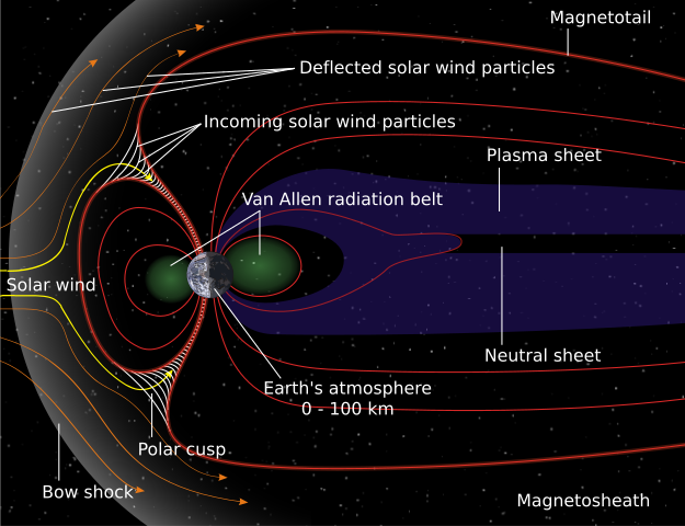
For life to form and survive depends on its complex molecules being protected from high-energy charged particles in the solar wind. In turn that depends on a strong geomagnetic field deflecting the solar wind as it does today, except for a small proportion that descend towards the poles and form aurora during solar mass ejections. In  visits to Isua in 2018 and 2019, geophysicists from the Massachusetts Institute of Technology, USA and Oxford University, UK drilled over 300 rock cores from metasedimentary ironstones (Nichols, C.I.O. and 9 others 2024. Possible Eoarchean records of the geomagnetic field preserved in the Isua Supracrustal Belt, southern West Greenland. Journal of Geophysics Research (Solid Earth), v. 129, article e2023JB027706; DOI: 10.1029/2023JB027706 Magnetisation preserved in the samples (remanent magnetism) suggest that it was formed by a geomagnetic field strength of at least 15 microtesla, similar to that which prevails today. The minerals magnetite (Fe3O4) and apatite (a complex phosphate) in the ironstones have been dated using U-Pb geochronometry and record a metamorphic event only slightly younger that the age of the Isua belt (3.69 and 3.63 Ga respectively). There is no sign of any younger heating above the temperatures that would reset the ironstones’ magnetisation. The Isua remanent magnetisation is at least 200 Ma older than that found in igneous rocks from north-eastern South Africa dated at between 3.2 to 3.45 Ga. So even in the Eoarchaean it seems likely that life, had it formed, would have avoided the hazard of exposure to the high energy solar wind. In all likelihood, however, in a shallow marine environment it would have had to protect itself somehow from intense ultraviolet radiation. That is now vastly reduced by stratospheric ozone (O3) which could only form once the atmosphere had appreciable oxygen (O2) content, i.e. after the Great Oxygenation Event beginning about 2.4 Ga ago. Undoubted stromatolites as old as 3.5 Ga suggest that early photosynthesising bacteria clearly had cracked the problem of UV protection somehow.

A companion crater for Chicxulub on the continental shelf of West Africa

Fig Interpreted 2D seismic section across the Nadir crater and central uplift beneath the Guinea Terrace. (Credit: Nicholson, et al. 2022. Fig 2c)

In 2022 four geoscientists from Heriot-Watt University in Edinburgh, Scotland and the Universities of Arizona and Texas (Austin), USA were geologically interpreting seismic-reflection data beneath the seafloor off Guinea and Guinea-Bissau, West Africa. Individual sedimentary strata that cover the upper continental crust show up as many reflectors. They are calibrated to rock cores from exploratory well that had revealed up to 8 km of sedimentary cover deposited continuously since the Upper Jurassic. The team’s objective was to collect information on tectonic structures that had formed when South America separated from Africa during the Cretaceous. The geophysical data were from commercial reconnaissance surveys aimed at locating petroleum fields beneath part of the West African continental shelf known as the Guinea Terrace. One of the seismic sections revealed a ~9 km wide basin-like depression at the level of the Cretaceous-Palaeogene boundary, which is underlain by a prominent upward bulge in reflectors corresponding to the mid-Cretaceous, plus a large number of nearby faults (Nicholson, U., and 3 others 2022. The Nadir Crater offshore West Africa: a candidate Cretaceous-Paleogene impact structure. Science Advances, v. 8, article eabn3096; DOI: 10.1126/sciadv.abn3096). Elsewhere on the Guinea Terrace the strata were featureless by comparison.

The Nadir crater showed many of the signs to be expected from an asteroid impact. That it drew attention stemmed partly from being of roughly the same age as the much larger 66 Ma Chicxulub impact off the Yucatan Peninsula of Mexico: the likely culprit for the K-Pg mass-extinction event. Perhaps both impactors stemmed from the break-up of a large, near-Earth asteroid because of gravitational forces resulting from a previous close encounter with either the Earth or another planet. The crater lies at the centre of a 23 km wide zone of faults that only affect Cretaceous and older strata; i.e. they formed just before the K-Pg event. The seismic data also show signs of widespread liquefaction of nearby Cretaceous sedimentary strata and that the crater had been filled by sediments shortly after it formed. Yet the data were too fuzzy for an astronomical catastrophe to be absolutely certain: similar structures can form from the rise of bodies of rock salt, which is less dense than sediments and will dissolve on reaching the seabed.  The owners of the seismic data donated a much larger collection from a grid of survey lines. Processing of such seismic grids turns the collection of individual two-dimensional sections into a 3D regional data set showing the complete shape of subsurface structures. Seismic data of this kind enables more detailed structural and lithological interpretation of both cross section and plan views. They enable sedimentary layers to be ‘peeled’ back to examine the crater at all depths, in much the same manner as CT  and MRI scans reveal the inner anatomy of the human body.

Map of faults around the Nadir crater at a level in the 3D seismic data that was about 200 m below the sea bed at the time of the impact. (Credit: Nicholson, et al. 2024, Fig 6)

Uisdean Nicholson and a larger team have now published their findings from the 3D seismic data that show the structure in unique detail (Nicholson, U., and 6 others 2024. 3D anatomy of the Cretaceous–Paleogene age Nadir Crater. Communications Earth & Environment v. 5, article number 547; DOI: 10.1038/s43247-024-01700-4). Nadir crater was affected by spiral-shaped thrust faults that suggest it was formed by an oblique impact from the northeast by an object around 450 m across, probably travelling at 20 km s-1 at 20 to 40° to the surface. Seconds after excavation uplift of deeper sediments was a response to removal of the load on the crust. The energy was sufficient to vaporise both sediment and impactor within a few seconds, the to drive drive seawater outwards in a tsunami about half a kilometre high, which in about 30 seconds exposed the incandescent crater floor. In the succeeding minutes hours and days liquefied sea water sloshed in and out of the crater, repeated tsunami resurgence forming gullies on its flanks and transporting sediment mixed with glass (suevite) flowed to refill the crater.

Time line for the Nadir impact, derived from detail shown by 3D seismic data. (Credit: Nicholson, et al. 2024, Fig 7)

There is no means of assigning any of the K-Pg extinctions to the Nadir crater, just that it happened at roughly the same time as Chicxulub. But it is the first impact crater to reveal the processes involved through complete coverage by high-resolution 3D seismic data. The majority of the roughly 200 craters are on the continental surface, and were thus ravaged to some extent by later erosion. Yet of the influx of hypervelocity objects through time at least 70% must have struck the oceans, but only 15 to 20 are known. That may reflect the fact that much deeper water could have buffered even giant impacts from affecting the oceanic crust beneath the abyssal plains, whose average depth is about 4 km. Only a small proportion of the continental shelves deemed to contain petroleum reserves have been explored seismically.  Chicxulub itself has been drilled, but only two seismic reflection sections have crossed its centre since its discovery, although earlier 3D data from petroleum exploration cover its outermost northern parts. More detail is available for Nadir and its lower energy did not smash its structural results, unlike Chicxulub. So, despite Nadir’s smaller size, fortuitously it gives more clues to how such marine craters formed. It looks to be an irresistible target for drilling.

A 9-day seismic reverberation set off by a giant tsunami in a Greenland fjord

In September 2023 the global network of seismic recorders detected a sequence of low-strength earth movements. It resembled the reverberation of a church bell albeit one that lasted for 9 days. rising and falling in strength every 90 seconds. For months this strange event on seismograms baffled geophysicists. All they could tell was that the signals did not show signs of having been generated by earthquakes; they were too regular. It was, however, possible to triangulate the position of the source of each individual event. There turned out to be only a single location for the seismic ‘campanology’ – at about 73° N on the eastern coast of Greenland, in Dickson Fjord and isolated branch of the enormous Kong Oscar Fjord system. Greenland is not noted for volcanic activity, ruling out the rumblings of a magma chamber that sometimes presages major eruptions. Whatever the cause, there were no human witnesses at the time. The only real clue lay at the start of the signal: the very long-period (VLP) signal was preceded by a sharp, high energy signal that could be matched with some kind of landslide.

View of a side glacier on Dickson Fjord, East Greenland where the tsunami occurred. Left – August 2023; right – 19 September 2023. The rocky peak at top centre on the left fell onto the glacier below to generate a rock-ice slide into the fjord. (Credit: Søren Rysgaard/Danish Army)

On 16 September 2023 the military base for the famous Sirius Dog Sled Patrol on Ella Island was smashed by a tsunami – fortunately it had been closed for the coming winter. When the Danish Navy patrolled Dickson Fjord some days later they found clear signs that the shores opposite the site of a recent colossal rock and ice slide (see images) had been scoured to a height of 200 m. For 5 km either side shoreline scouring averaged 60 m. The initial tsunami was gigantic, yet the fjord was able to contain its worst effects because the outlet to the rest of the system was at right angles to its trend. Some energy obviously was released to reach Ella Island near the mouth of the system to destroy the Danish Army post. The bizarre seismic signal was probably a result of the displaced water sloshing around in the fjord to dissipate the enormous energy released by the collapse of a mountain peak and a substantial amount of a valley glacier. Such behaviour is known as a seiche. Topographic analysis of Dickson Fjord enabled the researchers to calculate its resonant frequency: at 11 millihertz it matched that of the fluctuating seismic signal. (Svennevig, K. and 67 others 2024. A rockslide-generated tsunami in a Greenland fjord rang Earth for 9 days. Science, v. 385, p. 1196-1205; DOI: 10.1126/science.adm9247).

Valley glaciers in Greenland bolster their rocky flanks against collapse. With climatic warming being much faster there than for the rest of the world, its almost innumerable valley glaciers are shrinking. Yet they have been eroding the crust for tens of thousand years. The fjords that they occupied at the height of the last glacial maximum have very steep sides. Likewise, the remaining glaciers have carved U-shaped valleys. So when the glaciers retreat their exposed flanks become gravitationally unstable. Despite the fact that much of Greenland is underpinned by very hard crystalline rocks, that presents a major hazard for water craft. East Greenland’s spectacular scenery draws many tourist cruisers and Innuit fishing boats each summer. Moreover, removal of the ice load allows elastic strain that had built up in the upper crust to be released along joint systems that further weaken resistance to collapse.

A great deal of publicity has been given to the rapid melting of the huge ice sheet that covers most of Greenland. That is currently the biggest contributor to sea-level rise: a few millimetres per year. The Dickson Fjord event highlights the potential deadly threat of deglaciation, although the extremely complex nature of most of its fjord systems may prevent regional tsunamis from escaping their damping effect. Bu there are increasing dangers from the largest, more open fjords, such as Scoresby Sund, which conceivably might blurt catastrophic tsunamis towards Iceland, Svalbard and the west coast of Norway. Even small ones could wreak havoc on wildlife, such as seal and walrus nurseries.

See also: Carrillo-Ponce, A. et al. 2024. The 16 September 2023 Greenland Megatsunami: Analysis and Modeling of the Source and a Week‐Long, Monochromatic Seismic Signal. The Seismic Record, v. 4, p. 172-183; DOI: 10.1785/0320240013; Le Page, M. 2024. Greenland landslide caused freak wave that shook Earth for nine days. New Scientist 12 September 2024

Magnetic reversal and demise of the Neanderthals?

A rumour emerged last week that the Neanderthals met their end as one consequence of an extraterrestrial, possibly even extragalactic influence. Curiously, it stems from a recent discovery in New Zealand, where of course Neanderthals never set foot and nor did anatomically modern humans, the ancestors of Maori people, until a mere 800 years ago. It started with an ancient log from a kauri tree (Agathis australis), a species that Maoris revere. Found in excavations of boggy ground, the log weighed about 60 tons, so it was a valuable commodity, especially as it is illegal to fell living kauri trees. The wood is unaffected by burial and insect attack, has a regular grain and colour throughout, so is ideal for monumental Maori sculpture. Such swamp kauri also preserves their own life history in annual growth rings, and the log in question has 1700 of them. Using growth rings to chart climate variation gives the most detailed records of the recent past, provided the wood can be dated. Matching growth ring records from several trees of different ages is key to charting local climate with annual precision over several millennia.

An ancient kauri tree log recovered by swampland excavations in New Zealand. (Credit: Jonathan Palmer, in Voosen 2021)

Radiocarbon dating indicates that this particular kauri tree was growing around 42 thousand years ago. That is close to the upper limit for using 14C concentration in organic matter to determine age because the isotope has a short half-life (5730 years). In this case samples of the log would contain only about 0.7 % of its original complement of radioactive carbon. Cosmic rays generate 14C when they hit nitrogen atoms in the atmosphere and it enters COand thus the carbon cycle. Carbon dioxide taken up by photosynthesis to contribute carbon to plants contains only about one part per trillion of 14C. Consequently wood as ancient as that in the kauri log contains almost vanishingly small amounts, yet it can still be measured using mass spectrometry to yield an accurate radiometric age.

The particularly interesting thing about the 42 ka date is that it coincides with the timing of the last reversal of the Earth’s magnetic field, known as the Laschamps event. The kauri tree bears detailed witness through its growth rings to the environmental effects of a decrease in that field to almost zero as the poles flipped. The bulk of cosmic rays are normally deflected away from the Earth by the geomagnetic field, but during a reversal a great many more pass through the atmosphere, the most energetic reaching the surface and the biosphere. The kauri growth rings record fluctuations in the generation of 14C by their passage and thereby the geomagnetic field strength, which was only 6% of normal levels from 42.3 to 41.6 ka (Cooper, A. and 32 others  2021. A global environmental crisis 42,000 years ago. Science, v. 371, p. 811-818; DOI: 10.1126/science.abb8677). This coincided with an unrelated succession of periods of low solar activity and a reduced solar ‘wind’, which also provides some cosmic-rayprotection when activity is at normal levels; a ‘double whammy’. One consequence would have been destruction of stratospheric ozone by cosmic rays and thus increased ultraviolet exposure at ground level.

Combined with the highly precise growth-ring dating, the climatic changes over the 1700 year lifetime of the kauri tree can be linked to other records of environmental change. These include glacial ice- and lake-bed cores together with stalactite layers. Apparently, the Laschamps geomagnetic reversal coincided with abrupt shifts in wind belts and precipitation, perhaps triggering major droughts in the southern continents. Highly plausible, but some of the other speculations are less certain. For instance, some time around 42 ka, but far from well-established, Australia’s marsupial megafauna experienced major extinctions, the Neanderthals disappear from the fossil record and modern humans started decorating caves in Europe (20 ka after they did in Indonesia). In fact, speculation becomes somewhat silly, with suggestions that early Europeans went to live in caves because of increased exposure to UV (they knew, did they, while Neanderthals didn’t?), their painting and, by implication, their entire culture shifting through the shock and awe of mighty displays of the aurora borealis. Just because the number 42 is (or was), according to the late Douglas Adams’s Hitchhiker’s Guide to the Galaxy, ‘the answer to life, the universe and everything’, the authors tag the episode as the ‘Adams Event’. In their summary for The Conversation they include an animation with a quintessential Stephen Fry narrative, which Earth-logs readers can judge for themselves. Perhaps ‘Lockdown Trauma’ has a lot more to answer for, other than upsurges in Zoom conferences, knitting and gourmet experimentation …

See also: Voosen, P. 2021. Kauri trees mark magnetic flip 42,000 years ago. Science, v. 371, p. 766; DOI: 10.1126/science.371.6531.766

Hot-spot track beneath the Greenland ice cap

Around 63 Ma ago, during the Palaeocene Epoch, major igneous activity broke out in what are now both sides of the North Atlantic Ocean. After initial sputtering it culminated massively between 57 and 53 Ma. Relics are to be seen in Baffin Island, West and East Greenland, the Faeroes and north-western parts of the British Islands, in the form of flood basalts, dyke swarms and scattered remnants of central volcanoes. Offshore drilling on the North Atlantic’s continental shelves suggests that the volcanism extended over 1.3 million km2 and blurted out around 6.6 million km3 of magma. Not for nothing have the products of this event been categorised as a Large Igneous Province. Its formation took place before the North Atlantic existed. It began to form as this precursor magmatic paroxysm waned.  Continued basaltic magma production created the ocean floor each side of the mid-Atlantic Ridge system to divide North America and Greenland from northern Europe. Sea floor spreading continues, rising above sea level in Iceland, which is underlain by a large mantle plume.

The plume beneath Iceland may have been present at a fixed position in the mantle for tens of million years. A hot spot over which plate movements have shifted lithosphere to be heated in a similar way to a sheet of paper dragged slowly over a candle flame. The Iceland plume may have left a hot-spot track similar to that involved in the Hawaiian island chain. The ocean floor to the east and west of Iceland is shallower and forms broad rides at right angles to the trend of the Mid-Atlantic Ridge system, judged to be such tracks that are still warm and buoyant after formation over the plume. But are there traces of earlier passage of drifting lithosphere over the plume. A way to detect older hot-spot tracks is through variations in geothermal heat flow through the continental surface, a linear pattern raising suspicions of such trace of passage. There is no sign to the east beneath Europe, so what about to the west. Greenland, being mainly blanketed in ice, is not a good place to conduct such a search as it would involve deep drilling through the ice at huge cost for each hole. But there is a roundabout way of obtaining geothermal information without even setting foot on Greenland’s icy wastes.

The geomagnetic field measured at the surface records anomalies in rock magnetisation in the solid Earth beneath. Near-surface variations due to large variations in rock types that comprise the continental crust appear as sharp, high frequency signals. Aeromagnetic surveys over Greenland are characterised by such noisy patterns because the subsurface geology is extremely complicated. However, the underlying upper mantle beneath all continents is geologically quite bland, but being uniformly rich in iron it contains a high proportion of magnetic minerals such as magnetite (Fe3O4). The upper mantle should therefore leave a signal in the surface geomagnetic field, albeit a commensurately bland one. Like radio signals that span a large range of wavelengths, Earth properties that vary spatially, such as the geomagnetic field, may be analysed using filters. Once the high-frequency geomagnetic features of the crust are filtered out what should remain is a signal that reflects the magnetic structure of the upper mantle. It should be more or less featureless, yet beneath Greenland it isn’t.

greenland hot spot
Estimated Curie depth variation below Greenland (left) converted to geothermal heat flow variation (right). (Credit: Martos et al. 2018; Figures 1b and 1c)

Magnetic anomalies are created by magnetisation induced in magnetic minerals in rocks by the Earth’s magnetic field. Yet minerals lose their ability to be magnetised at temperatures above a threshold known as the Curie point, which is 580 °C for magnetite, the most abundant magnetic mineral. Depending on the geothermal heat flow the Curie point is exceeded at some depth in the lithosphere. So magnetic anomalies can safely be assumed to be produced only by rocks above the so-called Curie depth. Yasmina Martos of the British Antarctic Survey (now at the University of Maryland) and scientists from Britain, the US and Spain used a complex procedure, including gravity data and a few direct measurements of heat flow below Greenland as well as filtered aeromagnetic data, to estimate the variation in Curie depth beneath the ice cap. (Martos, Y.M. et al. 2018. Geothermal heat flux reveals the Iceland hotspot track underneath Greenland. Geophysical Research Letters, v. 45, online publication; doi: 10.1029/2018GL078289). Using that as an inverse proxy for heat flow they were able to map the likely geothermal variation beneath the island. Rather than a random and narrow variation in depth, as would be expected for roughly uniform heat flow, the Curie depth varied in a non-random way by over 20 km, equivalent to roughly 20 mW m-2.

The shallowest Curie depth and highest estimated heat flow occurs in East Greenland around Scoresby Sund where the largest sequence of Palaeocene flood basalts occur. It is also on a line perpendicular to the mid-Atlantic Rift system that meets the active Iceland plume. Running north-west from Scoresby Sund is a zone of locally high estimated heat flow. Martos et al. suggest that this is the track of Greenland’s motion over the Iceland hot spot from about 80 Ma to the period of maximum on-shore volcanism and the start of sea-floor spreading at around 50 Ma.

A fully revised edition of Steve Drury’s book Stepping Stones: The Making of Our Home World can now be downloaded as a free eBook

A new kind of seismology

The detection and analysis of earthquake waves has played a major role in the study of how the Earth works for more than a century. Seismology has laid bare the deep structure of our planet. Using records from seismographs that showed the arrival times at different sites of body waves propagated by a 1909 earthquake near Zagreb Croatian scientist Andrija Mohorovičić deduced that the upper Earth was layered. His name is given to the boundary between the crust and underlying mantle; the Mohorovičić Discontinuity (Moho for short). Applying the principles of wave reflection and refraction to wave-arrival times from major seismic events at seismographic stations across the Earth’s surface resulted in the discovery of deeper discontinuities in the mantle and the structure of the core. As the number of stations increased, largely as a result of the need to detect and pin-point tests of nuclear weapons, reversing the principles enabled the 3-D positions of lesser events to be plotted. The resulting swathes of seismicity defined the boundaries of tectonic plates, and from the varying depths at which earthquakes occurred came ideas about their nature; especially important for the mapping of subduction zones. Expansion and standardisation of the global seismographic network and the millions of records that it has produced, together with advances in their digital analysis, has created the current method of charting deep-Earth properties using seismic tomography. A remarkable outcome of such studies is the strikingly named ‘The Atlas of the Underworld’.

Up to now there has been a limit to the scope of such studies, particularly their resolution of features in the Earth’s mantle. Almost all the recording stations are on land, leaving the 70% of the surface covered by oceans devoid of data. Yet that might be set to change. The building of the Internet’s World Wide Web has largely depended on a growing network of telecommunications optic-fibre cables that criss-cross the oceans as well as the continents, stretching about a million kilometres. Using lasers at each end of a cable and interferometric analysis of two light signal that takes up a tiny proportion of the cable’s bandwidth it is possible to detect noise due to disturbances of the cable that result from earthquakes. On land this is compromised by local effects, such as traffic noise, but the ocean floors are remarkable quiet. Giuseppe Marra of Britain’s National Physical Laboratory discovered the potential of using optic fibre while testing a 79 km length cable linking atomic clocks at NPL and Reading (Marra, G. And 11 others 2018. Ultrastable laser interferometry for earthquake detection with terrestrial and submarine cables. Science online publication; doi:10.1126/science.aat4458). Purely by chance he observed unusually high spikes in noise during 2016. By no stretch of the imagination could they have been caused by events along the course of the cable. Curious, he eventually tracked the signals down to a series of earthquakes beneath Norcia in central Italy that cause death and destruction between 24 August and 30 October 2016. With a magnitude of 6.5, the last was the largest seismic event in Italy for 36 years. Subsequently, he and colleagues picked up the signal of a far less energetic event beneath the Mediterranean Sea (magnitude 3.4) from a cable linking Malta and Sicily.

F1.large
Map of submarine optic-fibre cables (credit: TeleGeography’s Telecom Resources)

With records from three suitably equipped cables an earthquake focus could be located precisely using triangulation. Together with the recorded signals, it would also be possible to use high magnitude earthquakes detected by optic-fibre cables to add to conventional seismic tomography, thereby sharpening the 3-D images of the deep Earth, which at present are plagued by blurring of much useful detail. Since both submarine and terrestrial cables might be used, such a method may become a bonanza for geophysicists

See also: Hand, E, 2018. Seafloor fibre optic cables can listen for earthquakes. Science, v. 360, p. 1160.

A fully revised edition of Steve Drury’s book Stepping Stones: The Making of Our Home World can now be downloaded as a free eBook

Large earthquakes and the length of the day

Geoscientists have become used to the idea that long-term global climate shifts are cyclical, as predicted by Milutin Milanković. The periods of shifts in the Earth’s orbital and rotational parameters are of the order of tens to hundreds of thousand years. The gravitational reasons why they occur have been known since the 1920s when Milanković came up with his hypothesis, and they were confirmed fifty years later. But there are plenty of other cycles with shorter periods. The last 115 years of worldwide records for earthquakes with magnitudes greater than 7 whose changing annual frequency shows a clear cyclical period of about 32 years. The records show peaks in 1910, 1943, 1970 and 2011 (see Bendick, R. & Bilham, R. 1917. Do weak global stresses synchronize earthquakes? Geophysical Research Letters, v. 44 online; doi/10.1002/2017GL074934). Unlike Milanković cycles, these oscillations were not predicted, but something synchronous with them must be forcing this behavior: a sort of “cross-talk”. Either global seismicity has a tendency for events to trigger others elsewhere on the Earth or some other process is periodically engaging with major brittle deformation to give it a nudge.

Rebecca Bendick, of the University of Montana, Missoula, and Roger Bilham of the University of Colorado, Boulder used a complex statistical method to check for synchronicity between the seismic cycles and other repetitive phenomena. It turns out that there is a close match with historic data for the length of the day which varies by several milliseconds. At first sight this may seem odd, until one realizes that day length is governed by the Earth’s speed of rotation (about 460 m s-1 at the Equator). The correlation is between increases in both major seismicity and the length of the day; i.e. quakes increase as rotation slows.  Day length can vary by a millisecond over a year or so during el Niño, which involves shifts of vast masses of Pacific Ocean water that affect rotation. But what of larger changes on a three-decade cycle? Seismic events and the forces that they release result from buildup of strain in the lithosphere, so the episodic earthquake maxima require some kind of transfer of momentum within the Earth. It does not need to be large, as the Milanković astronomical forcing of climate demonstrates, just a regular pulse.

One possibility is that, as rotation decelerates, decoupling between the liquid outer core and the solid mantle may change the flow of molten iron-nickel alloy.  That may be sufficient to transmit momentum and thus stress through the plastic mantle to the brittle lithosphere so that areas of high elastic strain are pushed beyond the rocks’ strength so that they fail. There are indeed signs that the geomagnetic field also changes with day length on a decadal basis (Voosen, P. 2017. Sloshing of Earth’s core may spike big quakes. Science, v. 358, p. 575; doi:10.1126/science.358.6363.575). Rotational deceleration began in 2011, and if the last century’s trend holds there may be an extra five large earthquakes next year. Could the deadly 7.3 magnitude earthquake at the Iran-Iraq border on 12 November 2017 be the start? If so, will the 32-year connection improve currently unreliable earthquake forecasting? Probably the best we can expect is increased global readiness. The study has nothing to add as regards which areas are at risk: although there is clustering in time there is none with location, even on the regional scale.

A fully revised edition of Steve Drury’s book Stepping Stones: The Making of Our Home World can now be downloaded as a free eBook


http://www.gettyimages.com/detail/news-photo/iranians-salvage-their-furniture-and-household-appliances-news-photo/874026786
Iranians salvage their furniture and household appliances from damaged buildings in the town of Sarpol-e Zahab in Iran’s western Kermanshah province near the border with Iraq, on November 14, 2017

Plate tectonic graveyard

Where do old plates go to die? For the most part, down subduction zones to mix with their original source, the mantle. Earth-Pages has covered evidence for quite a few of the dead plates, which emerges from a geophysical technique known as seismic tomography – analogous to X-ray or magnetic resonance scans of the whole human body. For 20 years geophysicists have been analysing seismograms from many stations across the globe for every digitally recorded earthquake, i.e. virtually all of those since the 1970s. This form of depth sounding goes far beyond early deep-Earth seismometry that discovered the inner and outer core, various transition zones in the mantle and measured the average variation with depth of mantle properties. Tomography relies on complex models of the paths taken by seismic body waves and very powerful computing to assess variations in the speed of P- and S-waves as they travelled through the Earth: the more rigid/cool the mantle is the faster waves travel through it and vice versa. The result is images of deep structure in 2-D slices, but the quality of such sections depends, ironically, on plate tectonics. Most earthquakes occur at plate boundaries. Such linearly distributed, one-dimensional sources inevitably leave the bulk of the mantle as a blur. Around 20 different methodologies have been developed by the many teams working on seismic tomography. So sometimes conflicting images of the deep Earth have been produced.

Results of seismic tomography across Central America showing anomalously fast (in blue) P- (top) and S-wave (bottom) speeds in map view at a fixed mantle depth (1290 km, left) and as vertical sections (right). The blue zones at right are interpreted to show a steeply dipping slab that represents subduction of the eastern Pacific Cocos plate since about 175 Ma ago (credit: van der Meer, D.G et al. ‘Atlas of the Underworld)

The technique has come of age now that superfast computing and use of multiple models have begun to resolve some of tomography’s early problems. The latest outcome is astonishing: ‘The Atlas of the Underworld’ catalogues 94 2-D sections from surface to the core-mantle boundary each of which spans 40° or arc – about a ninth of the Earth’s circumference (see: van der Meer, D.G., van Hinsbergen, D.J.J., and Spakman, W., 2017, Atlas of the Underworld: slab remnants in the mantle, their sinking history, and a new outlook on lower mantle viscosity, Tectonophysics online; doi.org/10.1016/j.tecto.2017.10.004). Specifically, the Atlas locates remnants of relatively cold slabs in the mantle that are suspected to be remnants of former subduction zones, or those that connect to active subduction. The upper parts of active slabs are revealed by the earthquakes generate along them. At deeper levels they are too ductile to have seismicity, so what form they take has long been a mystery. Once subduction stops, so do the telltale earthquakes and the slabs ‘disappear’.

The slabs covered by the ‘Atlas’ only go back as far as the end of the Permian, when the current round of plate tectonics began as Pangaea started to break-up. It takes 250 Ma for slabs to reach the base of the mantle and beyond that time they will have heated up and begun to be mixed into the lower mantle and invisible. Nevertheless, the rich resource allows models of vanished Mesozoic to Recent plates and the tectonics in which they participated, based on geological information, to be evaluated and enriched. Just as important, the project opens up the possibility of finding out how the mantle ‘worked’ since Pangaea broke up, in 3-D; a key to more than plate tectonics, including the mantle’s chemical heterogeneity. Already it has been used to estimate changes in the total length of subduction zones since 250 Ma ago, and thus arc volcanism and CO2 emissions, which correlates with estimates of past atmospheric CO2 levels, climate and even sea levels.

See also:  Voosen, P. 2016. ‘Atlas of the Underworld’ reveals oceans and mountains lost to Earth’s history. Science; doi:10.1126/science.aal0411.

Lee, H. 2017. The Earth’s interior is teeming with dead plates. Ars Technica UK, 18 October 2017.

Seismic menace of the Sumatra plate boundary

More than a decade after the 26 December 2004 Great Aceh Earthquake and the Indian Ocean tsunamis that devastating experience and four more lesser seismic events (> 7.8 Magnitude) have show a stepwise shift in activity to the SE along the Sumatran plate boundary. It seems that stresses along the huge thrust system associated with subduction of the Indo-Australian Plate that had built up over 200 years of little seismicity are becoming unlocked from sector to sector along the Sumatran coast. Areas further to the SE are therefore at risk from both major earthquakes and tsunamis. A seismic warning system now operates in the Indian Ocean, but the effectiveness of communications to potential victims has been questioned since its installation. However, increasing sophistication of geophysical data and modelling allows likely zones at high risk to be assessed.

Recent Great Earthquakes in different segments of the Sumatra plate margin (credit: Tectonics Observatory, California Institute of Technology http://www.tectonics.caltech.edu/outreach/highlights/sumatra/why.html

One segment is known to have experienced giant earthquakes in 1797 and 1833 but none since then. What is known as the Mentawai seismic gap lies between two other segments in which large earthquakes have occurred in the 21st century: it is feared that gap will eventually be filled by another devastating event. Geophysicists from the Institut de Physique du Globe de Paris and Nanyang Technological University in Singapore have published a high-resolution seismic reflection survey showing the subduction zone beneath the Mentawai seismic gap (Kuncoro, A.K. et al. 2015. Tsunamigenic potential due to frontal rupturing in the Sumatra locked zone. Earth and Planetary Science Letters, v. 432, p. 311-322). It shows that that the upper part of the zone, the accretionary wedge, is laced with small thrust-bounded ‘pop-ups’. The base of the accretionary wedge shows a series of small seaward thrusts above the subduction surface itself forming ‘piggyback’ or duplex structures.

Seismic reflection profile across part of the Sumatra plate boundary, showing structures produced by past seismicity. (credit: Kuncoro et al. 2015, Figure 3b)

The authors model the mechanisms that probably produced these intricate structures. This shows that the inactive parts of the plate margin have probably locked in stresses equivalent to of the order of 10 m of horizontal displacement formed by the average 5 to 6 cm of annual subduction of the Indo-Australian Plate over the two centuries since the last major earthquakes. Reactivation of the local structures by release of this strain would distribute it by horizontal movements of between 5.5 to 9.2 m and related 2 to 6.6 m vertical displacement in the pop-ups. That may suddenly push up the seafloor substantially during a major earthquake, thereby producing tsunamis. Whether or not this is a special feature of the Sumatra plate boundary that makes it unusually prone to tsunami production is not certain: such highly resolving seismic profiles need to be conducted over all major subduction zones to resolve that issue. What does emerge from the study is that a repeat of the 2004 Indian Ocean tsunamis is a distinct possibility, sooner rather than later.

The core’s influence on geology: how does it do it?

Although no one can be sure about the details of processes in the Earth’s core what is accepted by all is that changes in core dynamics cause the geomagnetic field to change in strength and polarity, probably through some kind of physical interaction between core and deep mantle at the core-mantle boundary (CMB). Throughout the last 73 Ma and especially during the Cenozoic Era geomagnetism has been more fickle than at any time since a more or less continuous record began to be preserved in the Jurassic to Recent magnetic ‘stripes’ of the world ocean floor. Moreover, they came in bursts: 5 in a million years at around 72 Ma; 10 in 4 Ma centred on 54 Ma; 17 over 3 Ma around 42 Ma; 13 in 3 Ma at ~24 Ma; 51 over a period of 12 Ma centring on 15 Ma. During the Late Jurassic and Early Cretaceous the core was similarly ‘busy’, the two time spans of frequent reversals being preceded by quiet ‘superchrons’ dominated by the same normal polarity as we have today i.e. magnetic north being roughly around the north geographic pole.

The Cenozoic history of magnetic reversals - black periods were when geomagnetic field polarity was normal and white when reversed. (credit: Wikipedia)
The Cenozoic history of magnetic reversals – black periods were when geomagnetic field polarity was normal and white when reversed. (credit: Wikipedia)

Until recently geomagnetic ‘flips’ between the two superchrons were regarded as random , perhaps suggesting chaotic behaviour at the CMB. But such a view depends on the statistical method used. A novel approach to calculating reversal frequency through time, however, shows peak-trough pairs recurring 5 times through the Cenozoic Era, approximately 13 Ma apart: maybe the chaos is illusory (Chane, J. et al. 2015. The 13 million year Cenozoic pulse of the Earth. Earth and Planetary Science Letters, v. 431, p. 256-263). So, here is a kind of yardstick to see if there may be any connection between core processes and those at the surface, which Chen of the Fujian Normal University, Fushou China and Canadian and Chinese colleagues compared with the very detailed Cenozoic oxygen-isotope (δ18O) record preserved by foraminifera in ocean-floor sediments, which is a well established proxy for changes in climate. Removing the broad trend of cooling through the Cenozoic resulted in a plot of more intricate climatic shifts that matches the geomagnetism record in both shape and timing of peak-trough pairs. It also turns out, or so the authors claim, that both measures correlate with changes in the rate of Cenozoic subduction of oceanic lithosphere (a measure of plate tectonic activity), albeit negative – peaks in magnetism and climate connecting with slowing in the pace of tectonics.

The analyses involved some complicated maths, but taken at face value the correlations beg the questions why and how? Long-term climate change contains an astronomical signal, encapsulated in the Milankovich hypothesis which has been tested again and again with little room for refutation. So is this all to do with gravitational influences in the Solar System. More exotic still is the possibility of 13 Ma cyclicity linking the Milankovich mechanism with the vaster scale of the Sun’s orbit oscillating through the disc of the Milky Way galaxy and theoretical hints of a mysterious role for dark matter in or near the galaxy. Or, is it a relationship in which climate and the magnetic field are modulated by plate tectonics through varying volcanic emissions of greenhouse gases and the deep effect of subduction on processes at the CMB respectively? To me that seems more plausible, but it is still as exceedingly complex as the maths used to reveal the correlations.

Continental hot-spot track in eastern Australia

cosgrove volcano track shown on map of australia
The Cosgrove volcanic track on a natural-colour image mosaic of Australia (credit: Drew Whitehouse, NCI National Facility VizLab)

It is sometimes forgotten that not only oceanic lithosphere provides evidence for hot spot tracks, probably because they are so obvious as island and seamount chains on bathymetric maps. They are not so clear on continents, either because of erosion of volcanoes or topography dominated by features that predate volcanism, but they account for about 20% of proposed tracks. Eastern Australia seems well endowed; four of them marked by a variety of volcanic structures that trend parallel to the Indo-Australian Plate’s NNE Cenozoic drift powered by the Southeast Indian Ridge that separates it from the Antarctic Plate. The timing of the volcanism along the proposed tracks is also highly persuasive. The longest of the tracks, extending about 2000 km SSW from Cape Hillsborough on the coast of central Queensland through New South Wales to Cosgrove in Victoria, is marked by sporadic volcanoes whose age decreases from Late Eocene in the north to Late Miocene in Victoria.

Unlike oceanic hot-spot tracks, those on continents are not continuous lines of volcanic occurrences. The Cosgrove track has several volcanic gaps, up to 650 km wide. This kind of patchy feature once encouraged hot-spot sceptics to question the tectonic affinities of what they regarded as fortuitous alignments. Where volcanic age trends consistent with the hypothesis emerged such doubts have faded into the background academic ‘noise’. In the case of the Cosgrove track all but one of the dates of volcanism tally quite well with the Cenozoic absolute motion of the Indo-Australian Plate and their position along the track (Davies, D.R. et al 2015. Lithospheric controls on magma composition along Earth’s longest continental hotspot track. Nature, v. 525, p. 511-514). Yet the objective of the authors, from the Australian National University and the University of Aberdeen in Britain, was not merely to establish the alignment as a hot-spot track, but to suggest what may have resulted in its marked patchiness.

The geochemistry of lavas from the volcanoes turns out to be of two fundamentally different types: ‘common-or-garden’ basalts in the case of Queensland and peculiar potassium-rich basalts containing the K-feldspathoid leucite in New South Wales and Victoria. Why these compositional differences occur where they do emerged very clearly when their positions were plotted on a new map of the thickness variations of the eastern Australian continental lithosphere. The ordinary basalts rest on the thinnest lithosphere (£110 km), whereas the leucitites are underlain by considerably thicker lithosphere (~135 km). This suggests that the rising mantle whose partial melting produced the magmas was halted at different depths, different geochemical ‘signatures’ of basalts depending on the pressure of melting. The most interesting outcome, albeit one based on an absence of evidence, is that the very large volcanic gaps along the track are each above much thicker lithosphere (>150 km). At those depths a rising mantle plume would be much less likely to begin melting.

Hotspots and plumes

One of the pioneers of plate tectonics, W. Jason Morgan, recognised in the 1970s that chains of volcanic islands and seamounts that rise from the ocean floor may have formed as the movement of lithospheric plates passed over sources of magma that lay in the mantle beneath the plates. He suggested that such hotspots were fixed relative to plate movements at the surface and likened the formation of chains such as that to the west of the volcanically active of the Hawaiian ‘Big Island’ to linear scorching of a sheet of paper moved over a candle flame. If true, it should be possible to use hotspots as a framework for the absolute motion of lithospheric plates rather than the velocities of individual plates relative to the others. But Morgan’s hypothesis has been debated ever since he formulated it. A test would be to see whether or not plumes of rising hot material in the deep part of the mantle can be detected. This became one of the first objectives of seismic tomography when it was devised in the last decade of the 20th century: a method that uses global earthquakes records to detect parts of the mantle where seismic waves traveled faster or slower than the norm: effectively patches of hot (probably rising) and cold rock. The first such evidence was equally hotly debated, one view being that the magma sources beneath oceanic islands such as Hawaii and Iceland were actually related to plate tectonics and that the hotspot hypothesis had become a kind of belief system.

English: global distribution of 45 identified ...
Global distribution of hotspots ( credit: Wikipedia)

The problem was that mantle plumes supposedly linked to magmatic hotspots in the upper mantle would be so thin that they would be difficult to detect even with seismic tomography. Geophysicists have been trying to sharpen up seismic resolution partly by using supercomputers to analyse more and more seismic records and also by improving the theory about how seismic waves interact with 3-D mantle structure. This has culminated in more believable visualisation of mantle structure (French, S.W. & Romanowicz, B. 2015. Broad plumes rooted at the base of the Earth’s mantle beneath major hotspots). The two researchers from the University of California at Berkeley in fact showed something different, but still robust support for Morgan’s 40-year old ideas. Instead of thin plumes, they have been able to show much broader conduits beneath at least 5 and maybe more active ends of hotspot chains. The zones extend upwards from the core-mantle boundary to about 1000 km below the Earth’s surface, where some bend sideways towards hotspots, perhaps as a result of another kind of upper mantle circulation.

Whole-Earth seismic tomography cross sections beneath a variety of volcanic islands, (Credit French and Romanowicz; http://www.nature.com/doifinder/10.1038/nature14876)

The sources of these hot columns at the core-mantle boundary appear to be zones of very low shear-wave velocities; i.e. almost, but not quite molten blobs. French and Romanowicz suggest that the columns are extremely long-lived and may even have a chemical dimension – as in the hypothesis of mantle heterogeneity. Another interesting feature of their results is that the striking vertical linearity of the columns could indicate that the overall motion of the lower mantle is extremely sluggish and punctured by discrete convection.

Thin- or thick-skinned tectonics: a test

How the continental lithosphere deforms at convergent plate margins has been a matter of opinion that depends on where observations have been made in ancient orogenic belts. One view is that arc and collisional orogens are dominated by deformation of the upper crust and especially the cover of sedimentary and volcanic rocks above deeper and older basement. This is a ‘thin-skinned’ model in which rocks of the upper crust are detached from those below and thicken more or less independently by thrust faulting, the formation of ductile nappes or a combination of the two. Mountain ranges, in this view, are the product of piling up of thrust slices or nappes, as exemplified by the Alps, Canadian Rockies and the Caledonian thrust belt of NW Scotland. Thick-skinned processes, as the name suggests, see crustal shortening and thickening as being distributed through the crust from top to bottom and even involving the lithospheric mantle. The hinterlands of both the Alps and the Scottish Caledonides show plenty of evidence for entire-crust deformation, deep crustal rocks being found sheared together with deformed rocks of the cover. It stands to reason that orogenic processes on the grand scale must involve a bit of both.

Both hypotheses stem from field work in deeply eroded, structurally complex segments of the ancient crust, and it is rarely if ever possible to say whether both operated together or one followed the other during the often lengthy periods taken by orogeny to reach completion, and the sheer scale of the process. Orogenesis is going on today, to which major seismic activity obviously bears witness. But erosion has not progress from cover through basement so, up to now, only seismicity and geodetic GPS measurements have been available to show that continental crust in general is being shortened and thickened, as well as being moved about. Potentially, a means of assessing active deformation, even in the deep crust, is to see whether or not the speeds of seismic waves at different depths are biased depending on their direction of travel. Such anisotropy would develop if the mineral grains making up rocks were deformed and rotated to preferred directions; a feature typical of metamorphic rocks. But to make such measurements on the scale of active orogens requires a dense network of seismometers and software that can tease directionality and depth out of the earthquake motions detected by it.

LS-tectonite from the Paraiba do Sul Shear Zon...
Aligned minerals in a Brazilian metamorphic rock (credit: Eurico Zimbres in Wikipedia)

A joint Taiwanese-American consortium set up such a network in Taiwan, which is capable of this type of seismic tomography. Taiwan is currently taking up a strain rate of 8.2 cm per year due to motion of the Philippine Plate on whose western flank the island lies: it is part of an island arc currently colliding with the stationary Eurasian Plate and whose crust is shortening. Results of seismic anisotropy (Huang, T.-Y. et al. 2015. Layered deformation in the Taiwan orogen. Science, v. 349, p. 720-723) show that the fast direction of shear (S) waves changes abruptly at about 10 to 15 km deep in the crust. In the upper crust this lines up with the roughly N-S structural ‘grain’ of the orogen. At between 13 to 17 km down there is no discernible anisotropy, below which it changes to parallel the direction of plate motion, ESE-WNW. It seems that thin skinned tectonics is indeed taking place, although probably not above a structural detachment. Simultaneously the deep crust is being deformed but the shearing is ascribed to the descent of lithospheric mantle of the Philippine Plate beneath the Eurasian Plate, while the deep crust remains attached to the upper crust. If it were possible to examine the mineral lineations now forming in both the Taiwanese upper and lower crust where metamorphism is active, then the two directions would be apparent. Although not mentioned by the authors, perhaps the detection of different directionality of aligned metamorphic minerals in low- and high-grade metamorphic rocks might indicate such tectonic processes in the past.

When Earth got its magnetic field

For a planet to produce life it needs various attributes. Exoplanet hunters tend to focus on the ‘Goldilocks’ Zone’ where solar heating is neither so extreme nor so little that liquid water is unstable on a planet’s surface. It also needs an atmosphere that retains water. Ultraviolet radiation emitted by a planet’s star dissociates water vapour to hydrogen and oxygen and the hydrogen escapes to space. The reason Earth has not lost water in this way is that little water vapour reaches the stratosphere because it is condensed or frozen out of the air as the lower atmosphere becomes cooler with altitude. Given moist conditions survivability to the extent that exists on Earth still needs another planetary parameter: the charged particles emitted as an interplanetary ‘wind ‘by stars must not reach the surface. If they did, their potential to break complex molecules would hinder life’s formation or wipe it out if it ventured onto land. A moving current of electrical charge, which is what a stellar ‘wind’ amounts to, can be deflected by a magnetic field. This is what happens on Earth, whose magnetic field is a good reason why our planet has supported life and its continual evolution since at least about 3.5 billion years ago.

Artist's rendition of Earth's magnetosphere.
Deflection of the solar ‘wind’ by Earth’s Earth’s magnetosphere. (credit: Wikipedia)

Direct proof of the existence of a geomagnetic field is the presence of aligned particles of magnetic minerals in rocks, for instance in a lava flow, caused by their acquiring magnetisation in a prevailing magnetic field once they cooled sufficiently. The earliest such remanent magnetism was found in igneous rocks from north-eastern South Africa dated at between 3.2 to 3.45 billion years. All older rocks do not show such a feature dating back to their formation because of thermal metamorphism that resets any remanent magnetism to match the geomagnetic field prevailing at the time of reheating. There are, however, materials that formed further back in time and are also known to resist thermal resetting of any alignments of magnetic inclusion. They are zircons (ZrSiO4), originally crystallised from igneous magmas, which may have locked in minute magnetic inclusions. Zircons are among the most change-resistant materials and they can also be dated with great precision, with the advantage that the U-Pb method used can distinguish between age of formation and that of any later heating. Famously, individual grains of zircon that had accumulated in an early Archaean conglomerate outcropping in the Jack Hills of Western Australia yielded ages going back from 3.2 to 4.4 billion years; far beyond the age of any tangible rock and close to the formation age of the Earth. Quite a target for palaeomagnetic investigations once a suitable technique had been developed.

Western Australia's Jack Hills
Western Australia’s Jack Hills from Landsat (credit NASA Earth Observatory)

John Tarduno and colleagues from the Universities of Rochester and California USA and the Geological Survey of Canada report the magnetic properties of the Jack Hills zircons (Tarduno, J.A. et al. 2015. A Hadean to Paleoarchean geodynamo recorded by single zircon crystals. Science, v. 349, p. 521-524). All of the grains analysed record magnetisation spanning the period 3.2 to 4.2 billion years that indicate geomagnetic field strengths ranging from that found today at the Equator to about an eighth of the modern value. So from 4.2 Ga onwards geomagnetism probably deflected the solar wind: the early Earth was set for living processes from its earliest days. The discovery also supports the likelihood of functioning plate tectonics during the Hadean.

Judging earthquake risk

The early 21st century seems to have been plagued by very powerful earthquakes: 217 greater than Magnitude 7.0; 19 > Magnitude 8.0 and 2 >Magnitude 9.0. Although some lesser seismic events kill, those above M 7.0 have a far greater potential for fatal consequences. Over 700 thousand people have died from their effects: ~20 000 in the 2001 Gujarat earthquake (M 7.7); ~29 000 in 2003 Bam earthquake (M 6.6); ~250 000 in the 2004 Indian Ocean tsunami that stemmed from a M 9.1 earthquake off western Sumatra; ~95 000 in the 2005 Kashmir earthquake (M7.6); ~87 000 in the 2008 Sichuan earthquake (M 7.9); up to 316 000 in the 2010 Haiti earthquake (M 7.0); ~20 000 in the 2011 tsunami that hit NE Japan from the M 9.0 Tohoku earthquake. The 26 December 2004 Indian Ocean tsunamis spelled out the far-reaching risk to populated coastal areas that face oceans prone to seismicity or large coastal landslips, but also the need for warning systems: tsunamis travel far more slowly than seismic waves and , except for directly adjacent areas, there is good chance of escape given a timely alert. Yet, historically http://earthquake.usgs.gov/earthquakes/world/most_destructive.php, deadly risk is most often posed by earthquakes that occur beneath densely populated continental crust. Note that the most publicised earthquake that hit San Francisco in 1906 (at M 7.8) that lies on the world’s best-known fault, the San Andreas, caused between 700 and 3000 fatalities, a sizable proportion of which resulted from the subsequent fire. For continental earthquakes the biggest factor in deadly risk, outside of population density, is that of building standards.

English: A poor neighbourhood shows the damage...
A poor neighbourhood in Port au Prince, Haiti following the 2010 earthquake measuring >7 on the Richter scale. (credit: Wikipedia)

It barely needs stating that earthquakes are due to movement on faults, and these can leave distinct signs at or near to the surface, such as scarps, offsets of linear features such as roads, and broad rises or falls in the land surface. However, if they are due to faulting that does not break the surface – so-called ‘blind’ faults – very little record is left for geologists to analyse. But if it is possible to see actual breaks and shifts exposed by shallow excavations through geologically young materials, as in road cuts or trenches, then it is possible to work out an actual history of movements and their dimensions. It has also become increasingly possible to date the movements precisely using radiometric or luminescence means: a key element in establishing seismic risk is the historic frequency of events on active faults. Some of the most dangerous active faults are those at mountain fronts, such as the Himalaya and the American cordilleras, which often take the form of surface-breaking thrusts that are relative easy to analyse, although little work has been done to date. A notable study is on the West Andean Thrust that breaks cover east of Chile’s capital Santiago with a population of around 6 million (Vargas, G. Et al. 2014. Probing large intraplate earthquakes at the west flank of the Andes. Geology, v. 42, p. 1083-1086). This fault forms a prominent series of scarps in Santiago’s eastern suburbs, but for most of its length along the Andean Front it is ‘blind’. The last highly destructive on-shore earthquake in western South America was due to thrust movement that devastated the western Argentinean city of Mendoza in 1861. But the potential for large intraplate earthquakes is high along the entire west flank of the Andes.

Vargas and colleagues from France and the US excavated a 5 m deep trench through alluvium and colluvium over a distance of 25 m across one of the scarps associated with the San Ramon Thrust. They found excellent evidence of metre-sized displacement of some prominent units within the young sediments, sufficient to detect the effects of two distinct, major earthquakes, each producing horizontal shifts of up to 5 m. Individual sediment strata were dateable using radiocarbon and optically stimulated luminescence techniques. The earlier displacement occurred at around 17-19 ka and the second at about 8 ka. Various methods of estimation of the likely earthquake magnitudes of the displacements yielded values of about M 7.2 to 7.5 for both. That is quite sufficient for devastation of now nearby Santiago and, worryingly, another movement may be likely in the foreseeable future.

New gravity and bathymetric maps of the oceans

By far the least costly means of surveying the ocean floor on a global scale is the use of data remotely sensed from Earth orbit. That may sound absurd: how can it be possible to peer through thousands of metres of seawater? The answer comes from a practical application of lateral thinking. As well as being influenced by lunar and solar tidal attraction, sea level also depends on the Earth’s gravity field; that is, on the distribution of mass beneath the sea surface – how deep the water is and on varying density of rocks that lie beneath the sea floor. Water having a low density, the deeper it is the lower the overall gravitational attraction, and vice versa. Consequently, seawater is attracted towards shallower areas, standing high over, say, a seamount and low over the abyssal plains and trenches. Measuring sea-surface elevation defines the true shape that Earth would take if the entire surface was covered by water – the geoid – and is both a key to variations in gravity over the oceans and to bathymetry.

Radar altimeters can measure the average height of the sea surface to within a couple of centimetres: the roughness and tidal fluctuations are ‘ironed out’ by measurements every couple of weeks as the satellite passes on a regular orbital schedule. There is absolutely no way this systematic and highly accurate approach could be achieved by ship-borne bathymetric or gravity measurements, although such surveys help check the results from radar altimetry over widely spaced transects. Even after 40 years of accurate mapping with hundreds of ship-borne echo sounders 50% of the ocean floor is more than 10 km from such a depth measurement (80% lacks depth soundings)

This approach has been used since the first radar altimeter was placed in orbit on Seasat, launched in 1978, which revolutionised bathymetry and the details of plate tectonic features on the ocean floor. Since then, improvements in measurements of sea-surface elevation and the computer processing needed to extract the information from complex radar data have show more detail. The latest refinement stems from two satellites, NASA’s Jason-1(2001) and the European Space Agency’s Cryosat-2 (2010) (Sandwell, D.T. et al. 2014. New global marine gravity model from CryoSat-2 and Jason-1 reveals buried tectonic structure. Science, v. 346. p. 65-67; see also Hwang, C & Chang, E.T.Y. 2014. Seafloor secrets revealed. Science, v. 346. p. 32-33). If you have Google Earth you can view the marine gravity data by clicking here.  The maps throw light on previously unknown tectonic features beneath the China Sea (large faults buried by sediments), the Gulf of Mexico (an extinct spreading centre) and the South Atlantic (a major propagating rift) as well as thousands of seamounts.

Global gravity over the oceans derived from Jason-1 and Cryosat-2 radar altimetry (credit: Scripps Institution of Oceanography)

There are many ways of processing the data, and so years of fruitful interpretation lie ahead of oceanographers and tectonicians, with more data likely from other suitably equipped satellites: sea-surface height studies are also essential in mapping changing surface currents, variations in water density and salinity, sea-ice thickness, eddies, superswells and changes due to processes linked to El Niño.

Signs of lunar tectonics

Large features on the near side of the Moon give us the illusion of the Man-in-the-Moon gazing down benevolently once a month. The lightest parts are the ancient lunar highlands made from feldspar-rich anorthosite, hence their high albedo. The dark components, originally thought to be seas or maria, are now known to be large areas of flood basalt formed about half a billion years after the Moon’s origin. Some show signs of a circular structure and have been assigned to the magmatic aftermath of truly gigantic impacts during the 4.1-3.8 Ga Late Heavy Bombardment. The largest mare feature, with a diameter of 3200 km, is Oceanus Procellarum, which has a more irregular shape, though it envelopes some smaller maria with partially circular outlines.

Full Moon view from earth In Belgium (Hamois)....
Full Moon viewed from Earth. Oceanus Procellarum is the large, irregular dark feature at left. (credit: Wikipedia)

A key line of investigation to improve knowledge of the lunar maria is the structure of the Moon’s gravitational field above them. Obviously, this can only be achieved by an orbiting experiment, and in early 2012 NASA launched one to provide detailed gravitational information: the Gravity Recovery and Interior Laboratory (GRAIL) whose early results were summarised by EPN in December 2012. GRAIL used two satellites orbiting in a tandem configuration similar to the US-German Gravity Recovery and Climate Experiment (GRACE) launched in 2002 to measure variations over time in the Earth’s gravity field. The Grail orbiters flew in a low orbit and eventually crashed into the Moon in December 2012, after producing lots of data whose processing continues.

The latest finding from GRAIL concerns the gravity structure of the Procellarum region (Andrews-Hanna, J.C. and 13 others 2014. Structure and evolution of the lunar Procellarum region as revealed by GRAIL gravity data. Nature, v. 514, p. 68-71) have yielded a major surprise. Instead of a system of anomalies combining circular arcs, as might be expected from a product of major impacts, the basaltic basin has a border made up of many linear segments that define an unusually angular structure.

The topography and gravity structure of the Moon. Oceanus Procellarum is roughly at the centre. Note: the images cover both near- and far side of the Moon. (credit: Andrews-Hanna et al 2014)

The features only become apparent from the gravity data after they have been converted to the first derivative of the Bouguer anomaly (its gradient). Interpreting the features has to explain the angularity, which looks far more like an outcome of tectonics than bombardments. The features have been explained as rift structures through which basaltic magma oozed to the surface, perhaps feeding the vast outpourings of mare basalts, unusually rich in potassium (K), rare-earth elements (REE) and phosphorus (P) know as KREEP basalts. The Procellarum polygonal structure encompasses those parts of the lunar surface that are richest in the radioactive isotopes of potassium, thorium and uranium (measured from orbit by a gamma-ray spectrometer) – thorium concentration is shown in the figure.

Tectonics there may be on the Moon, but the authors are not suggesting plate tectonics but rather structures formed as a huge mass of radioactively heated lunar lithosphere cooled down at a faster rate than the rest of the outer Moon. Nor are they casting doubt on the Late Heavy Bombardment, for there is no escaping the presence of both topographic and gravity-defined circular features, just that the biggest expanse of basaltic surface on the Moon may have erupted for other reasons than a huge impact.

Tectonics of the early Earth

Tectonics on any rocky planet is an expression of the way heat is transferred from its deep interior to the surface to be lost by radiation to outer space. Radiative heat loss is vastly more efficient than either conduction or convection since the power emitted by a body is proportion to the fourth power of its absolute temperature. Unless it is superheated from outside by its star, a planet cannot stay molten at its surface for long because cooling by radiation releases all of the heat that makes its way to the surface.  Any football supporter who has rushed to get a microwaved pie at half time will have learned this quickly: a cool crust can hide a damagingly hot centre.

Thermal power is delivered to a planet’s surface by convection deep down and conduction nearer the surface because rocks, both solid and molten, are almost opaque to radiation. The vigour of the outward flow of heat might seem to be related mainly to the amount of internal heat but it is also governed by limits imposed by temperature on the form of convection. Of the Inner Planets only Earth shows surface signs of deep convection in the form of plate tectonics driven mainly by the pull exerted by steep subduction of cool, dense slabs of old oceanic lithosphere. Only Jupiter’s moon Io shows comparable surface signs of inner dynamics, but in the form of immense volcanoes rather than lateral movements of slabs. Io has about 40 times the surface heat flow of Earth, thanks largely to huge tidal forces imposed by Jupiter. So it seems that a different mode of convection is needed to shift the tidal heat production; similar in many ways to Earth’s relatively puny and isolated hot spots and mantle plumes.

Most of the yellow and orange hues of Io are d...
An analogy for the early Earth, Jupiter’s moon Io is speckled with large active volcanoes; signs of vigorous internal heat transport but not of plate tectonics. Its colour is dominated by various forms of sulfur rather than mafic igneous rocks. (credit: Wikipedia)

Shortly after Earth’s accretion it would have contained far more heat than now: gravitational energy of accretion itself; greater tidal heating from a close Moon and up to five times more from internal radioactive decay. The time at which plate tectonics can be deduced from evidence in ancient rocks has been disputed since the 1970s, but now an approach inspired by Io’s behaviour approaches the issue from the opposite direction: what might have been the mode of Earth’s heat transport shortly after accretion (Moore, W.B. & Webb, A.A.G. 2013. Heat-pipe Earth. Nature, v.  501, p. 501-505). The two American geophysicists modelled Rayleigh-Bénard convection – multicelled convection akin to that of the ‘heat pipes’ inside Io – for a range of possible thermal conditions in the Hadean. The modelled planet, dominated by volcanic centres turned out to have some surprising properties.

The sheer efficiency of heat-pipe dominated heat transfer and radiative heat lost results in development of a thick cold lithosphere between the pipes, that advects surface material downwards. Decreasing the heat sources results in a ‘flip’ to convection very like plate tectonics. In itself, this notion of sudden shift from Rayleigh-Bénard convection to plate tectonics is not new – several Archaean specialists, including me, debated this in the late 1970s – but the convincing modelling is. The authors also assemble a plausible list of evidence for it from the Archaean geological record: the presence in pre- 3.2 Ga greenstone belts of abundant ultramafic lavas marking high fractions of mantle melting; the dome-trough structure of granite-greenstone terrains; granitic magmas formed by melting of wet mafic rocks at around 45 km depth, extending back to second-hand evidence from Hadean zircons preserved in much younger rocks. They dwell on the oldest sizeable terranes in West Greenland (the Itsaq gneiss complex), South Africa and Western Australia (Barberton and the Pilbara) as a plausible and tangible products of ‘heat-pipe’ tectonics. They suggest that the transition to plate-tectonic dominance was around 3.2 Ga, yet ‘heat pipes’ remain to the present in the form of plumes so nicely defined in the preceding item Mantle structures beneath the central Pacific.

Mantle structures beneath the central Pacific

Since it first figured in Earth Pages 13 years ago seismic tomography has advanced steadily as regards the detail that can be shown and the level of confidence in its accuracy: in the early days some geoscientists considered the results to be verging on the imaginary. There were indeed deficiencies, one being that a mantle plume which everyone believed to be present beneath Hawaii didn’t show up on the first tomographic section through the central Pacific. Plumes are one of the forms likely to be taken by mantle heat convection, and many now believe that some of them emerge from great depths in the mantle, perhaps at its interface with the outer core.

The improvements in imaging deep structure stem mainly from increasingly sophisticated software and faster computers, the data being fed in being historic seismograph records from around the globe. The approach seeks out deviations in the speed of seismic waves from the mean at different depths beneath the Earth’s surface. Decreases suggest lower strength and therefore hotter rocks while abnormally high speeds signify strong, cool parts of the mantle. The hotter mantle rock is the lower its density and the more likely it is to be rising, and vice versa.

Using state-of-the-art tomography to probe beneath the central Pacific is a natural strategy as the region contains a greater concentration of hot-spot related volcanic island chains than anywhere else and that is the focus of a US-French group of collaborators (French, S. et al. 2013. Waveform tomography reveals channeled flow at the base of the oceanic lithosphere. Science, v. 342, 227-230;  doi 10.1126/science.1241514). The authors first note the appearance on 2-D global maps for a depth of 250 km of elongate zones of low shear-strength mantle that approximately parallel the known directions of local absolute plate movement. The most clear of these occur beneath the Pacific hemisphere, strongly suggesting some kind of channelling of hot material by convection away from the East Pacific Rise.

Seismic tomograhic model of the mantle beneath the central Pacific. Yellow to red colours represent increasing low shear strength. (credit: Global Seismology Group / Berkeley Seismological Laboratory
Seismic tomographic model of the mantle beneath the central Pacific. Yellow to red colours represent increasingly low shear strength. (credit: Global Seismology Group / Berkeley Seismological Laboratory)

Visually it is the three-dimensional models of the Pacific hot-spot ‘swarm’ that grab attention. These show the low velocity zone of the asthenosphere at depths of around 50 to 100 km, as predicted but with odd convolutions. Down to 1000 km is a zone of complexity with limb-like lobes of warm, low-strength mantle concentrated beneath the main island chains. That beneath the Hawaiian hot spot definitely has a plume-like shape but one curiously bent at depth, turning to the NW as it emerges from even deeper mantle then taking a knee-like bend to the east . Those beneath the hot spots of the west Pacific are more irregular but almost vertical. Just what kind of process the peculiarities represent in detail is not known, but it is almost certainly a reflection of complex forms taken by convection in a highly viscous medium.

Probing the Earth’s mantle using noise

sesmic tomography
Artistic impression of a global seismic tomogram – beneath Mercator projection – dividing the mantle into ‘warm’ and ‘cool’ regions (Credit: Cornell University Geology Department – http://www.geo.cornell.edu/geology/classes/Geo101/graphics/s12fsl.jpg)

It goes without saying that it is difficult to sample the mantle. The only direct samples are inclusions found in igneous rocks that formed by partial melting at depth so that the magma incorporated fragments of mantle rock as it rose, or where tectonics has shoved once very deep blocks to the surface. Even if such samples were not contaminated in some way, they are isolated from any context. For 20 years geophysicists have been analysing seismograms from many stations across the globe for every digitally recordable earthquake to use in a form of depth sounding. This seismic tomography assesses variations in the speed of body (P and S) waves according to the path that they travelled through the Earth.

Unusually high speeds at a particular depth suggests more rigid rock and thus cooler temperatures whereas hotter materials slow down body waves. The result is images of deep structure in vertical 2-D slices, but the quality of such sections depends, ironically, on plate tectonics. Earthquakes, by definition mainly occur at plate boundaries, which are lines at the surface. Such a one-dimensional source for seismic tomograms inevitably leaves the bulk of the mantle as a blur. But there are more ways of killing a cat than drowning it in melted butter. All kinds of processes unconnected with tectonics, such as ocean waves hitting the shore and interfering with one another across the ocean basins, plus changes in atmospheric pressure especially associated with storms, also create waves similar in kind to seismic ones that pass through the solid Earth.

Such aseismic energy produces the background noise seen on any seismogram. Even though this noise is way below the energy and amplitude associated with earthquakes, it is continuous and all pervading: the cumulative energy. Given highly sensitive modern detectors and sophisticated processing much the same kind of depth sounding is possible using micro-seismic noise, but for the entire planet and at high resolution. Rather than imaging speed variations this approach can pick up reflections from physical boundaries in the solid Earth. Surface micro-seismic waves exactly the same as Rayleigh and Love waves from earthquakes have already been used to analyse the Mohorovičić discontinuity between crust and upper mantle as well as features in the continental crust; indeed the potential of noise was recognized in the 1960s. But the deep mantle and core are the principle targets, being far out of reach of experimental seismic surveys using artificial energy input. It seems they are now accessible using body-wave noise (Poli, P. et al. 2012. Body-wave imaging of Earth’s mantle discontinuities from ambient seismic noise. Science, v. 338, p. 1063-1065).

Poli and colleagues from the University of Grenoble, France and Finland used a temporary network of 42 seismometers laid out in Arctic Finland to pick up noise, and sophisticated signal processing to separate surface waves from body waves. Their experiment resolved two major mantle discontinuities at ~410 and 660 km depth that define a transition zone between the upper and lower mantle, where the dominant mineral of the upper mantle – olivine – changes its molecular state to a more closely packed configuration akin to that of the mineral perovskite that is thought to characterize the lower mantle. Moreover, they were able to demonstrate that the 2-step shift to perovskite occupies depth changes of about 10-15 km.

Applying the method elsewhere doesn’t need a flurry of new closely-spaced seismic networks. Data are already available from arrays that aimed at conventional seismic tomography, such as USArray that deploys  400 portable stations in area-by-area steps across the United States (http://earth-pages.co.uk/2009/11/01/the-march-of-the-seismometers/)

It is early days, but micro-seismic noise seems very like the dreams of planetary probing foreseen by several science fiction writers, such as Larry Niven who envisaged ‘deep radar’ being deployed for exploration by his piratical hero Louis Wu. Trouble is, radar of that kind would need a stupendous power source and would probably fry any living beings unwise enough to use it. Noise may be a free lunch to the well-equipped geophysicist of the future.

  • Prieto, G.A. 2012. Imaging the deep Earth. Science (Perspectives), v. 338, p. 1037-1038.

The shuffling poles

The mechanical disconnection of the lithosphere from the Earth’s deep mantle by a more ductile zone in the upper mantle – the asthenosphere – suggests that the lithosphere might move independently. If that were the case then points on the surface would shift relative to the axis of rotation and the magnetic poles, irrespective of plate tectonics.  So it makes sense to speak of absolute and relative motions of tectonic plates. The second relates to plates’ motions relative to each other and to the ancient position of the magnetic poles, assumed to be reasonably close to that of the past pole of rotation, yet measurable from the direction of palaeomagnetism retained in rocks on this or that tectonic plate. Plotting palaeomagnetic pole positions through time for each tectonic plate gives the impression that the poles have wandered. Such apparent polar wandering has long been a key element in judging ancient plate motions.  Absolute plate motion judges the direction and speed of plates relative to supposedly fixed mantle plumes beneath volcanic hot spots, the classic case being Hawaii, over which the Pacific Plate has moved to leave a chain of extinct volcanoes that become progressively older to the west. But it turns out that between about 80 to 50 Ma there are some gross misfits using the hot-spot frame of reference. An example is the 60° bend of the Hawaiian chain to become the Emperor seamount chain that some have ascribed to hot spots shifting (see http://earth-pages.co.uk/2009/05/01/the-great-bend-of-the-pacific-ocean-floor/).

English: Age of ocean floor, with fracture zon...
Age of Pacific Ocean floor, showing the Hawaii-Emperor seamount chain in black. (credit: Wikipedia)

Ideas have shifted dramatically since it became clear that hot spots can shift, and there has been an attempt to estimate their actual motions (Doubrovine, P.V. et al. 2012. Absolute plate motions in a reference frame defined by moving hot spots in the Pacific, Atlantic, and Indian oceans. Journal of Geophysics Research: Solid Earth, v. 117, B09101, doi:10.1029/2011JB009072). It is early days for the revised view of absolute motion of the lithosphere and estimates go back only 120 Ma. However, one outcome has been a realistic examination of whether the positions of the poles have shifted through time; a possibility that is hidden in apparent polar wander paths. Since the mid-Cretaceous it seems that a slow and hesitant, but significant polar shuffle has taken place, varying between 0.1 and 1.0° Ma-1, starting in one direction and then the movement retraced its steps to achieve the current proximity of magnetic poles to the poles of rotation.

Geophysics reveals secrets of the beaver

Beaver Hut
Beaver lodge and dam (Photo credit: Bemep)

One of the interesting things about the beaver is that its obsession with civil engineering may have a profound effect upon landscape. Before Europeans set foot in North America, it is estimated that up to 400 million of them inhabited the continent. The ponds that they create by building the dams in which they live securely, encourage sedimentation. It is quite possible that this creates recognisable stratigraphic formations; but no-one really knows as active and wet beaver habitats hide what lies beneath them. It is clearly urgent to obtain this intelligence: the Geological Society of America’s monthly Geology contained in its first issue for 2012 a paper that indeed probes the legacy of large rodents long gone (Kramer, N. et al. 2012. Using ground penetrating radar to ‘unearth’ buried beaver dams. Geology, v. 40, p. 43-46).

The target for surveillance was the eponymous Beaver Meadows in Colorado, USA, and not only did the researchers from Colorado State University deploy ground-penetrating radar, but used the seismic reflection method as well, to quantify volumes of beaver-induced sedimentation. Fortunately, despite their past presence in some strength, beavers no longer frequent Beaver Meadows and no ethical lines in the sand were crossed. Beaver and elk seemingly have long competed for the meagre resources of Beaver Meadows, the rodent having finally succumbed locally to determined efforts by the elk to consume the beavers’ victuals. As disconcerted and no doubt sulking beavers failed to maintain their dams and lodges, the water table fell, further encouraging the elk. Eventually, at some time after the Beaver Survey of 1947, the last of them moved to new meadows. Their ravages (see http://animal.discovery.com/videos/fooled-by-nature-beaver-dams.html) of what would otherwise be dense woodland have, however, made it possible for geophysicists to try out their sophisticated kit on a new and thorny issue: they ran 6 km of GPR and seismic profiles.

I came across this handsome animal (Castor can...
A beaver. Image via Wikipedia

In much the same way as larger scale geophysical data are interpreted for petroleum traps, signs of hydrocarbons, mighty listric faults and zones of tectonic inversion, the beaver-oriented sections potentially yield considerable insight to the trained eye. There are indeed beaverine sedimentary aggradations of Holocene age above the local glacial tills. Beneath Beaver Meadow they amount to as much as 50% of post-glacial sediment. Apparently, the deposits have a linear element that follows the local drainages.

Seafloor mud cores and the seismic record

Chikyu
Japan's deep-sea Drilling Vessel "CHIKYU" Image via Wikipedia

The most important factors in attempting to assess risk from earthquakes are their frequency and the time-dependence of seismic magnitude. Historical records, although they go back more than a millennium, do not offer sufficient statistical rigor for which tens or hundreds of thousand years are needed. So the geological record is the only source of information and for most environments it is incomplete, because of erosion episodes, ambiguity of possible signs of earthquakes and difficulty in precise dating; indeed some sequences are extremely difficult to date at all with the resolution and consistency that analysis requires. One set of records that offer precise, continuous timing is that from ocean-floor sediment cores in which oxygen isotope variations related to the intricacies of climate change can be widely correlated with one another and with the records preserved in polar ice cores. For the past 50 ka they can be dated using radiocarbon methods on foraminifera shells The main difficulty lies in finding earthquake signatures in quite monotonous muds, but one kind of feature may prove crucial; evidence of sudden fracturing of otherwise gloopy ooze (Sakagusch, A. et al. 2011. Episodic seafloor mud brecciation due to great subduction zone earthquakes. Geology, v.39, p. 919-922).

The Japanese-US team scrutinised cores from the Integrated Ocean Drilling Program (IODP) that were drilled 5 years ago through the shallow sea floor above the subduction zone associated with the Nankai Trough to the SE of southern Japan. Young, upper sediments were targeted close to one of the long-lived faults associated with the formation of an accretionary wedge by the scraping action of subduction. Rather than examining the cores visually the team used X-ray tomography similar to that involved in CT scans, which produce precise 3-D images of internal structure. This showed up repeated examples of sediment disturbance in the form of angular pieces of clay set in a homogeneous mud matrix separated by undisturbed sections containing laminations. The repetitions are on a scale of centimetres to tens of centimetres and were dated using a combination of 14C and 210Pb dating (210Pb forms as a stage in the decay sequence of 238U and decays with a half-life of about 22 years, so is useful for recent events). The youngest mud breccia gave a 210Pb age of AD 1950±20, and probably formed during the 1944 Tonankai event, a great earthquake with Magnitude 8.2. Two other near-surface breccias gave 14C ages of 3512±34 and 10626±45 years before present. These too probably represent earlier great earthquakes as it can be shown that mud fracturing and brecciation by ground shaking needs accelerations of around 1G, induced by earthquakes with magnitudes greater than about 7.0. So, not all earthquakes in a particular segment of crust would show up in seafloor cores, most inducing turbidity flow of surface sediment, but knowing the frequency of the most damaging events, both by onshore seismicity and tsunamis, could be useful in risk analysis. In its favour, the method requires cores that penetrate only about 10 m, so hundreds could be systematically collected using simple piston coring rigs where a weighted tube is dropped onto the sea floor from a small craft.

Core’s comfort blanket and stable magnetic fields

Pangea animation
Pangaea and its break-up. Image via Wikipedia

The record of the Earth’s magnetic field for the most part bears more than a passing resemblance to a bar-code mark, by convention black representing normal polarity, i.e. like that at the present, and white signifies reversed polarity. The bar-code resemblance stems from long periods when the geomagnetic poles flipped on a regular, short-term basis, by geological standards. The black and white divisions subdivide time as represented by geomagnetic into chrons of the order of a million-years and subchrons that are somewhat shorter intervals. Stemming from changes in the Earth’s core, magnetostratigraphic divisions potentially occur in any sequence of sedimentary or volcanic igneous rocks anywhere on the planet and so can be used as reliable time markers; that is, if they can be defined by measurements of the remanent magnetism preserved in rock, which is not universally achievable. Yet this method of chronometry is extremely useful, for most of the Phanerozoic. However, there were periods when the geomagnetic field became unusually stable for tens of million years so the method is not so good. These have become known as superchrons, of which three occur during Phanerozoic times: the Cretaceous Normal Superchron when the field remained as it is nowadays from 120 to 83 Ma; a 50 Ma long period of stable reversed polarity (Kiaman Reverse Superchron) from 312 to 262 Ma in the Late Carboniferous and Early Permian; the Ordovician Moyero Reverse Superchron from 485 to 463 Ma.

Because the geomagnetic field is almost certainly generated by a self-exciting dynamo in the convecting  liquid metallic outer core, polarity flips mark sudden changes in how heat is transferred through the outer core to pass into the lower mantle. It follows that if there are no magnetic reversals then the outer core continued in a stable form of convection; the likely condition during superchrons. But why the shifts from repeated instability to long periods of quiescence? That is one of geoscience’s ‘hard’ questions, since no-one really knows how the core works at any one time, let alone over hundreds of million years. There is however a crude correlation with events much closer to the surface. The Kiaman superchron spans a time when Alfred Wegener’s supercontinent Pangaea had finished assembling so that all continental material was in one vast chunk. The Cretaceous superchron was at a time when sea-floor spreading and the break-up of Pangaea reached a maximum. The Ordovician, Moyero superchron coincides with the unification of what are now the northern continents into Laurasia and the continued existence of the southern continents lumped in Gondwana, so that the Earth had two supercontinents. Those empirical observations may have been due to chance, but at least they provide a possible clue to linkage between lithosphere and core, despite their separation by 2800 km of convecting mantle that transfers the core heat as well as that produced by the mantle itself to dissipate at the surface. Enter the modellers.

How part of the Earth transfers heat is, not unexpectedly, very complex, depending not only on what is happening at that point but on heat-transfer processes and heat inputs both above and below it. The surface heat flow is complex in its own right ranging from less than 20 to as much as 350 mW m-2, the largest amount being through zones of sea-floor spreading and the least  through continental lithosphere. Wherever heat is released in the core and mantle, willy-nilly the bulk of it leaves the solid Earth along what is today a complex series of lines; active oceanic ridge and rift systems such as the mid-Atlantic Ridge.  These lines weave between six drifting continental masses and many more sites of additional heat loss – hot spots and mantle plumes. The many heat escape routes today complicate the deeper convective processes and there are many possibilities for the core to shed heat, yet they continually change pace and position. When, inevitably, all continental lithosphere unites in a supercontinent, almost by definition, the sites of heat loss simplify too, the supercontinent acting like an efficient insulating blanket. In a qualitative sense, this kind of evolving scenario is what modellers try to mimic by putting in reasonable parameters for all the dynamic aspects involved.  Two physicists at the University of Colorado in Boulder, USA, Nan Zhang and Shije Zhong, have formulated 3-D spherical models of mantle convection with plate tectonics as a basis for whole Earth thermal evolution over that last 350 Ma (Zhang, N & Zhong, S. 2011.  Heat fluxes at the Earth’s surface and core–mantle boundary since Pangea formation. Earth and Planetary Science Letters, v. 306, p. 205-216). The acid test is whether the model can end with a close approximation to modern variations in heat flow and distribution of ages on the sea floor; it does. A probable key to stability in the means of transfer of heat from core to lower mantle – itself a key to a constant outer-core dynamo and geomagnetic polarity – is reduced heat flow at equatorial latitudes; a sort of equatorial downflow of convection with upflows in both northern and southern hemispheres. Zhang and Zhong’s model produced minimal core-to-mantle heat flow at  the Equator at 270 and 100 Ma, both within geomagnetic-field superchrons. Well, that is a good start. Superchrons seem also to have occurred from time to time during the Precambrian, one being documented at the Mesoproterozoic-Neoperoterozoic boundary about 1000 Ma ago. At that time, all continental lithosphere was assembled in a supercontinent dubbed Rodinia (‘homeland’ or ‘birthplace’ in Russian).

Bulges that move

In 2008 a team of geophysicists from Cambridge University, UK published an astonishingly detailed picture of about 500 km2 of a land surface complete with drainage systems (Figure 3 in Rudge, J.F. et al. 2008. A plume model of transient diachronous uplift at the Earth’s surface. Earth and Planetary Science Letters, v. 267, p. 146-160). The surprise was not its Palaeogene age (~55  Ma), but that it is buried beneath the Atlantic continental shelf about 200 km west of the Shetland Isles and had been revealed by detailed, 3-D seismic reflection surveys during oil exploration. Technically it is buried landscape unconformity that resulted from uplift (by almost 500 m) and erosion (for ~1.3 Ma) that interrupted Palaeocene to Eocene marine sedimentation and was suddenly buried to preserve the details of river channels: uplift rapidly gave way to subsidence and conditions returned to marine about 0.6 Ma later. The timing and the location of such a transient crustal bulge, during the early part of opening of the North Atlantic, suggests that it stemmed from a thermal source, probably the Iceland hot spot straddled by the mid-Atlantic Ridge. The model favoured by the authors is radially horizontal spreading of a pulse of especially hot mantle outwards from the plume beneath the Iceland hot spot; a ‘plume head’. Volumetric expansion of the lithosphere causes the uplift, and movement away from the plume of the hot mantle results in an annular, outward moving ripple. Cooling once the thermal source has passed produces subsidence.

The idea clearly has ‘legs’ for a whole number of reasons, not the least being the sheer number of long-lived hot spots above mantle plumes that affect the ocean basins and parts of the continents, Africa and North America especially. Now it has been publicised more widely than in a specialised journal (Williams, C. 2011. Pulsating planet. New Scientist, v. 209 (12 March 2011), p. 41-43). One of the original authors is reported to have suggested that the ~55 Ma thermal ripple beneath the nascent North Atlantic may have destabilised gas hydrates in the sediments causing methane to belch out in its wake. That is a possible mechanism for the Palaeocene-Eocene thermal maximum and its huge associated carbon isotope ‘spike’ likely stemming from boosted atmospheric methane.

Grand Canyon
The Grand Canyon from the South Rim. Image via Wikipedia

Probably the most famous extant bulge is the one through which the Colorado River has carved the USA’s 1.8 km deep Grand Canyon: the Colorado Plateau. Long believed to have formed above hot, low-density lithosphere too, this uplift is the subject of completely new ideas that also have stemmed in part from seismic data, though not produced by artificial reflectance methods. Geophysicists in the US have developed a system that uses hundreds of transportable seismometers that are being ‘marched’ from west to east as an array that uses seismographs from natural earthquakes world-wide to perform seismic tomography –3-D mapping of varying seismic velocities and thereby rigidity and density in the mantle – with improved resolution because of the close spacing of the recording stations. Publications from the Earthscope USarray are beginning to appear from the western USA, one of which concerns the Colorado Plateau (Levander, A.et al, 2011. Continuing Colorado plateau uplift by delamination-stylee convective lithospheric downwelling. Nature, v. 472, p. 461-465). The western part of the plateau is associated with a high-velocity anomaly that extends to around 90m km beneath, which the authors ascribe to a large blob of rigid mantle that has detached from the lithosphere and is slowly sinking. This ‘drip’ is an example of delamination where mantle that becomes detached from the lithosphere causes it to thin and reduces its overall density. The overlying crust rises in response. There is a thermal effect, as warmer, less rigid asthenosphere convects upwards to fill the gap left by the drip, but it is an effect rather than a cause of the uplift.

See also: Zandt, G. & Reiners, P. 2011. Lithosphere today… Nature, v. 472, p. 420-421.