Climate change reducing Earth’s albedo

According to a new study (Goode, P. R.et al. 2021. Earth’s albedo 1998–2017 as measured from earthshine. Geophysical Research Letters, v. 48, article e2021GL094888; DOI: 10.1029/2021GL094888) the ability of the Earth to reflect solar radiation back into space has been decreasing significantly over the last two decades. The conclusion has arisen from measurements of the brightness of the lunar surface. A new Moon is barely visible, apart from a thin sliver illuminated by the Sun. Its overall faint brightness is due to sunlight reflected from the Earth’s surface that faces the Moon: so-called ‘earthshine’. New Moons occurs when it is above the lit side of the Earth, so they appear during daylight hours. Earthshine depends on the ability of the Earth’s surface and cloud cover to reflect solar radiation, or its albedo. Albedo was high during the last ice age because of continental ice sheets and it can also occur when there is an unusually large percentage of cloud cover or a lot of dust and aerosols in the atmosphere, perhaps after a large volcanic eruption. High albedo leads to global cooling. Decreased albedo allows the atmosphere to heat up, and conspires with the greenhouse effect to produce global warming.

Philip Goode and his colleagues measured earthshine on the Moon between 1998 and 2017 to precisely determine daily, monthly, seasonal, yearly and decadal changes in terrestrial albedo. The Earth reflects roughly 30% of the solar energy that falls on it, although it varies with Earth’s rotation, depending on the proportion of land to ocean that is sunlit. Over the two decades earthshine decreased gradually by ~0.5 W m-2, indicating a 0.5% decrease in Earth’s albedo and a corresponding increase in the amount of solar energy received at the land and ocean surfaces. To put this in perspective the estimated warming from anthropogenic greenhouse emissions over the same period increased by just a little more (0.6 W m-2). Albedo decrease is reinforcing the greenhouse effect.

Sea-surface temperature anomalies over the Pacific Ocean during a ‘positive’ phase of the Pacific Decadal Oscillation – reversal to a ‘negative’ phase cools the eastern Pacific and warms the west (Credit: Wikipedia)

Although it might seem that increased seasonal melting of polar sea ice would have the main effect on albedo, this is not borne out by the earthshine data. What is strongly implicated is a decrease over the Eastern Pacific Ocean of highly reflective low-altitude clouds. That might seem counterintuitive, since warming of the sea surface increases evaporation, but the reduced low-cloud cover has been measured from satellites. Many scientists and most climate-change deniers have thought that an increase in cloud cover at low latitudes and thus albedo would moderate surface warming. The opposite seems to be happening. The key may lie in one of the Earth’s largest climate phenomena, the Pacific Decadal Oscillation (PDO). This has a major effect on global climate through long-distance connections (teleconnections) to other climatic processes. The satellite data hint at the changes in albedo of the Western Hemisphere having been related to a long-term reversal in the PDO. The Earth’s climate system increasingly reveals its enormous complexity.

See also: Earth is dimming due to climate change, Science Daily, 30 September 2021.

The risk of landslides in Africa

The most widespread risk from natural hazards is, with little doubt, that posed by ground instability; landslides and landslips; mudflows; rock avalanches and a range of other categories in which large volumes of surface material are set in motion. They can be triggered by earthquakes, volcanism or heavy rainfall that changes the physical properties of rock and soil. Not only steep slopes pose a risk, for some affect ground with quite gentle topography, as witness the terrible scenes from Sulawesi triggered by the 28 September 2018 magnitude 7.5 earthquake beneath the Minhasa Peninsula. This set in motion mudflows on gently sloping ground when the seismic waves caused liquefaction of unconsolidated sediments that not only shattered dwellings by the lateral motion, but whole communities sank into the slurry with little trace. The rapid events left a death toll confirmed at 2010 people with about 5000 missing, feared to have been swallowed by the earth. In the last 9 months mass movement has resulted in fatalities in many places, the most publicised being in Uganda, Japan, Philippines, Sulawesi, Ethiopia, Sumatra, South India, Bangladesh, California, Nepal, and the list grows as it does every year.

407458aa.2
Types of mass movement (Credit: US Geological Survey

As well as purely natural causes, human activities, such as deforestation, excavations and dumping of materials, greatly exacerbate risks. The South Wales former coal-mining communities commemorate every year the collapse of a mine spoil heap on a steep hillside on 21 October 1966 that engulfed a primary school at Aberfan, killing 116 small children and 28 adults. Wherever they occur, there seems to be little chance of escape for those in their path. Slowly it has become possible for geoscientists to outline areas that are potentially at risk from catastrophic mass wastage, sometimes from the distribution of scars of previous events on remotely sensed images, but increasingly by multivariate analysis of landscapes in terms of the factors that may contribute to future ground failures. The principal ones are: topographic slope and relief; annual rainfall, especially the likely precipitation in a single day; vegetation cover, particularly by trees; strength of surface rock and soils, including degrees of consolidation, interbedding and water content; geological structure, such as the trajectory of faults, degree of  jointing and the dip of strata. Modelling risk has to grapple with the global scale of the problem, which cannot be addressed in the least developed regions by piecemeal local studies, although those are urgent, of course, in areas with recorded instances of catastrophic ground failure. Regional studies can screen vast areas of probably low risk so that meagre resources can focus on those that appear to be most dangerous to populated places.

afr landslide
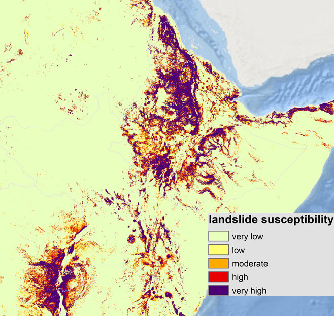
Degree of risk from landslides of all types in the northern part of the East African Rift System (Credit: Broeckx et al. 2018; Fig. 6)

Belgian engineering geologists and GIS specialists have assembled a monumental risk assessment of Africa, together with a bibliography of all published work on mass movement across the continent (Broeckx, J. et al. 2018. A data-based landslide susceptibility map of Africa. Earth-Science Reviews, v. 185, p. 102-121; DOI: 10.1016/j.earscirev.2018.05.002). They point out that Google Earth’s 3-D viewing potential at fine spatial resolution provides a free and rapid means of mapping scars of previous earth movements in considerable detail over areas that data analysis suggests to be susceptible. Their paper provides continent-scale maps of the parameters that they used as well as maps showing several versions of their risk analysis. The supplementary data to the paper include downloadable, full-resolution maps of landslide susceptibility.

German global DEM now freely available

407458aa.2
TerraSAR-X and Tandem-X satellites fly close to each other some 500km above the Earth

In  2007 and 2010 two radar-imaging satellites were launched by the German space agency DLR, TerraSAR-X and Tandem-X respectively. After 2010 both orbited in close, side-by-side formation, sometimes as little as 200 m apart. With one acting as a both a transmitter and receiver of microwave pulses, the other as a receiver, this set up allowed the two signals returning from the Earth’s surface to be matched. The slightly different positions of the platforms results in a time difference at which a pulse reflected from a point on the Earth’s surface reaches the two receiving antennas. This difference varies according to the topographic elevation of the point – in effect analogous to the parallax shift captured in conventional stereoscopic images but measured by the interference between the two signals. Although involving far more complex computation, such radar interferometry produces estimates of each point’s elevation and ultimately a 3-dimensional image of the Earth’s surface. After a period of commercial operation, DLR has decided to make part of the data available free of charge. Both systems use microwaves with a wavelength of around 3 cm (9.65 GHz frequency), which allows topographic elevation to be measured to a precision of ±1 m. Using orbits that cross the poles, each at an angle to the Equator, allows swaths from the dual system eventually to cover the whole planet, in the manner of winding a ball of string. Eventually, the data will permit the detection of vertical movements of one kind or another when multiple coverage of the Earth becomes available. However, the expected lifetime of the platforms is limited, so DLR plans to launch two 23.6 cm interferometric radar satellites to assess dynamic processes occurring on the Earth’s surface.

407458aa.2
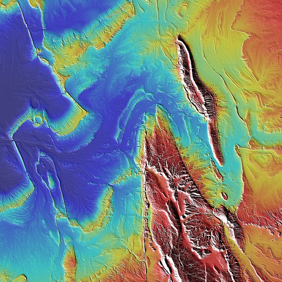
Side illuminated, colour-coded TanDEM-x elevation model of part of the Sahara desert, in the Tamanrasset province of central Algeria

The resolution of radar interferometry in the two dimensions of a map depends on many factors, some of which stem from the complex processing of the raw data. DLR global data is presented at three resolutions (pixel size): 12 m, the finest; 30 m and 90 m. For local acquisition even finer resolution is possible. Only the 90 m version is being released for free use. The first interferometric radar elevation data to be made freely available was from the NASA Shuttle Radar Topography Mission (SRTM) that was accomplished from the US Space Shuttle Endeavour in 2000, using a single instrument that incorporated two antennas separated by a 60 m long mast deployed from the Shuttle. SRTM acquired data only between latitudes 60° N and 60° S, using 23.6 cm L-band radar. As well as omitting high latitudes, the SRTM design limited actual elevation precision to about 4 m compared with the ±1 m from TerraSAR-X/TanDEM-X. SRTM data with a two-dimensional resolution of 30 m are freely available from the US Geological Survey.

Full global elevation data with a 30 m 2-D resolution and elevation precision of ±9 m have also been produced by the optical stereoscopic potential of the US-Japan ASTER imaging system and are freely available to all via the US Geological Survey. Unlike data produced by radar missions, the optical stereoscopic data from ASTER depend on cloud-free, daytime conditions, and accurate derivation of parallax can be prevented by areas of rugged terrain in deep shadow at the 10 am local-time when images are acquired.

Despite the limitation of TerraSAR-X/TanDEM-X elevation data to a 90 m 2-D resolution, and the consequent loss of textural detail in landscapes, they appear to have the edge in terms of completeness and vertical precision. To get elevation data from DLR requires personal registration after reading a lengthy screed of documentation about data acquisition.

Ice cliffs on Mars

An illustration of what Mars might have looked...
An illustration of what Mars might have looked like during an ice age between 2.1 million and 400,000 years ago, when Mars’s axial tilt is believed to have been much larger than today.  (credit: Wikipedia)

For Mars to support life and for life to have emerged there demand water that is readily accessible from the surface. There is evidence that in the distant past liquid water may have flowed across the Martian surface to erode river-like features, some associated with the vast canyon system of Valles Marineris. That feature is thought to have been initiated by tectonic forces and perhaps flowing magma, but it shows definite signs of water erosion. Water in great volume was released during the Noachian phase of Mars’s evolution possibly by major impacts 4100 to 3700 million years ago, during the interval known as the Late Heavy Bombardment). Large tracts of the Martian surface that are more muted than Valles Marineris show topographic features reminiscent of huge braided stream systems. Water may have covered vast, low-lying areas in the planet’s Northern Hemisphere to form an early ocean. Yet today the Red Planet seems extremely dry and its thin atmosphere shows only minute traces of water vapour – it is dominated by carbon dioxide. Results from various rovers deployed across its surface and from Mars orbiting satellites have, however, revealed signs of waterlain sediments and minerals that can only have formed by the breakdown of igneous rocks by water. Signs that liquid water continues to flow occasionally down steep slopes, such as rill-like features and ephemeral darkened patches, have been much disputed.

Mars does have an ice cap at its North Pole that waxes and wanes with its seasons, but rather than melting during Martian ‘summers’ the ice sublimates directly to water vapour. Conversely, the polar ices probably form from frost. Yet, astonishingly, there appear to be active glaciers complete with flow lines and moraines, but chances are that some of them are sediment flows ‘lubricated’ by frost binding together mineral particles and boulders that undergoes pressure-induced regelation. Data from orbiting neutron and gamma-ray spectrometers reveal that between 60°N and 60°S the top metre of Martian soil contains between 2 to 18% of ice, making it akin to terrestrial permafrost. So, contrary to its appearance Mars is rich in water, but almost exclusively in solid form. Until very recently, the bulk was thought to be as a matrix binding together sediments, accessible to future crewed mission in useful volumes only by surface mining. That somewhat pessimistic view has now changed dramatically.

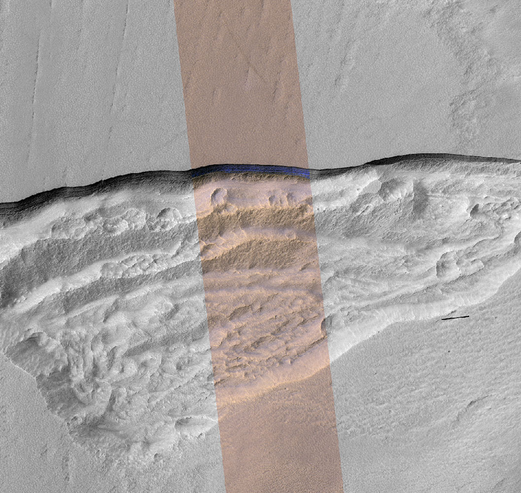
Monochrome HiRISE image of a cliff on Mars (the pinkish swath is a simulated natural colour image – see below). beneath the cliff is a zone of jumbled ground formed by cliff collapses. (credit: NASA)

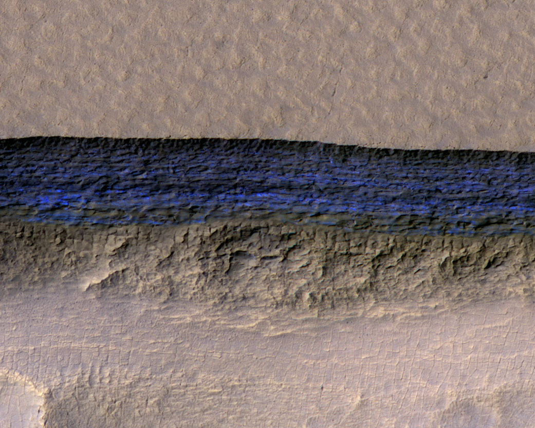
Careful study of fine resolution imagery from the HiRISE instrument on the Mars Reconnaissance Orbiter at latitudes a little less than 60° has centred on cliffs formed by recent erosion (Dundas, C.M and 11 others 2018. Exposed subsurface ice sheets in the Martian mid-latitudes. Science, v. 359, p. 199-201; doi: 10.1126/science.aao1619). Colin Dundas of the US Geological Survey, Flagstaff, Arizona, and US colleagues used the multispectral capacities of HiRISE data to study the composition of sedimentary layers exposed in the cliffs. In eight cases, the cliffs contained layered, almost pure blue ice tens of metres thick and only a few metres below the surface. The cliffs seem to have formed as ice has sublimated where exposed, thereby undermining to sedimentary cover. Below the cliffs are jumbled zones of collapsed material. Being so close to the surface and underlain by apparently ice-free sediments, the layered ice sheets must be geologically quite young.

Simulated natural-colour HiRISE image of a Martian cliff showing nearly pure water ice in blues. Note the layered structure that may represent seasonal variations during the period of ice formation (credit: NASA)

Unlike the Earth, whose axial tilt is stabilised to a large degree by the Moon’s gravity, Mars’s two tiny moons have little effect of this kind. So Mars’s axis wobbles between its current 25° tilt to as much as 45°. This results in large climatic shifts, of which there have been an estimated forty over the last 5 million years. At high tilts solar energy heats up the poles and releases water vapour by accelerated sublimation to be laid down at lower latitudes as frost or snow. Mars’s present tilt suggests that it is experiencing a cold episode so that wind blown dust has covered and preserved mid-latitude ice sheets over tens of thousand years. Nearly pure ice is easier to exploit than permafrost layers. Yet optimism among enthusiasts for a crewed Mars mission and eventual colonisation is tempered by the latitudes of the discoveries. While ready supplies of water from ice and CO2 from the Martian atmosphere give the ingredients for oxygen, methane through catalysis of CO2 and hydrogen, agricultural photosynthesis and all kinds of other useful chemistry, low latitudes offer the most assured solar energy supplies. Latitudes around 55° are frigid and dark during Martian winters; perhaps totally inhospitable. So the remote-sensing search is likely to continue in cliffs closer to the ‘tropics’ of Mars.

Developments in remotely sensed data for geology

Over several decades remote sensing – the interpretation and analysis of image data – has become a central part of many geologists’ ‘toolkit’. It continues a ‘tradition’ founded in the interpretation of panchromatic (black and white), stereoscopic aerial photographs that began after World War 2. But after 1972 and the launch of the first Landsat platform, it has been served by more synoptic views from space using a variety of systems that produce data in many wavelengths of EM radiation, thereby providing opportunities to study spectral properties of the Earth’s surface. This imagery also possesses the analytical flexibility afforded by being recorded in digital form. Since the 1986 launch of the first SPOT platform digital stereoscopic potential from space entered the options for geological interpretation. The Landsat Thematic Mapper (TM) launched in 1982 expanded the spectral range of data. Previously that had been restricted to the visible and near infrared (VNIR) affected mainly by living vegetation and the iron oxy-hydroxides that are the main colorants of rock and soil and TM added a shortwave infrared (SWIR) band. Natural reflectance spectra in that region are affected by Al-OH, Mg-OH and C-O bonds in various hydroxylated silicates and carbonate minerals. The data from TM and its successor the Enhanced Thematic Mapper (ETM) resulted in an explosion of effort into lithological mapping and structural analysis. The last depended on a step-change in resolution to 15 m in the panchromatic band of the ETM system since 1993, together with 10 m stereoscopic resolution from the SPOT family, that enable confident mapping at around 1:100 000 to 1:50 000 scales.

The ETM, its successor on Landsat-8 in 2013 – the Operational Land Imager (OLI) – and the somewhat similar ESA Sentinel-2 system (2015) suffer from one major frustration. Their single broad SWIR band is unable to discriminate –OH and C-O spectral features and hence the lithologically useful range of hydroxylated silicates and carbonate mineral spectra. Also missing from the spectral ‘toolkit’ was any data relating to the major rock-forming silicates. Both drawbacks were remedied to some extent by the launch in 1999 of the Japan/US Advanced Spaceborne Thermal Emission and Reflection Radiometer (ASTER). As well as the VNIR in three bands, including a stereo-image pair, this covered the mineralogically useful SWIR with 6 narrow  wavelength range bands imaging and 5 bands in the thermally emitted infrared (TIR) where common silicates show substantial spectral differences. ASTER produced primarily geoscientific data that have been found to be of enormous use in geological and mineralogical mapping at the 1:100 000 scale.

Nowadays all the data types mentioned so far, except SPOT, are available for download free of cost from the Earth Explorer site operated by the US Geological Survey (use the Data Sets tab at the EE home page): a superb resource that would suit most geological applications. Yet none of these data have spatial resolution better than 10 m. The commercial Earth observation sector has mainly focussed on increasingly finer spatial resolution, mainly panchromatic and the VNIR range of wavelengths that yield information on vegetation and surface topographic and cultural detail, for which there are many profitable markets. Apart from the follow-on to SPOT – the Pléiades system with resolution as fine as 0.5 m – data from a whole constellation of once independent hi-res systems (WorldView, Quickbird, GeoEye, IKONOS and OrbView) are now administered by one vendor Digital Globe. The finest resolution currently available publically is that of WorldView-3 (0.3 m), beyond which is the classified purview of the US intelligence community. The figure illustrates just how much more detailed geological information there is in the finest resolution data than in the same kind of image reduced to 15 m resolution, the best offered by ASTER. That detail needs to be tempered by a few facts: by comparison with the high-res image ASTER shows a regional context, i.e. large-scale geological structures; it covers more spectral bands and is therefore more revealing lithologically; the highest resolution data (WorldView-3 archived) are priced at US$14 to 19 per km2  for each of 6 different band-bundles with a minimum order of 25 km2. Note: for some areas Google Earth has coverage at high-resolution captured at several dates, though some remain at 15 m resolution (based on Landsat-7 ETM).

30cm v 15m
An area in Utah, USA, with almost 100% exposure and very low vegetation cover shown by simulated natural colour images at ~0.3 m with a scale of ~1:1225 (top) and ~15 m at ~1:61275. Credit: Google Earth

The geologist’s dream data would, I suppose, consist of many bands that divide the VNIR, SWIR and TIR into narrow wavebands so that rock and soil spectra can be accurately reproduced, thereby allowing considerable discrimination between different rock types and their main constituent minerals. Oh yes, and it would have decent resolution – better than 15 m. There is indeed such a hyperspectral instrument called CRISM and data from it can be downloaded freely but, before there is a stampede to get access, note that the acronym stands for Compact Reconnaissance Imaging Spectrometer for Mars! For the Earth most hyperspectral data are captured from airborne missions, except for one orbital mission that occasionally functioned over a tiny fraction of the Earth from 2001 to 2017 – NASA’s EO-1 Hyperion system that produced 7.5 km swaths at 30 m resolution with 220 spectral bands covering the VNIR and SWIR regions. Apart from one aimed at oceanic and atmospheric issues, that will say little about rocks, NASA and ESA have no plans in this niche. One commercial developer, Satellogic of Argentina, has hyperspectral plans but only where an income stream is guaranteed, which seems to be just for crops and vegetation spanning the VNIR range. Other outfits have wish lists but few concrete plans in the geoscientific spectral range.

With pending budget cuts to NASA’s Earth science programme (9%), NOAA (22%) and the USGS (14%) demanded by the Trump administration, progress with US contributions to Earth observation can’t be anticipated with much hope. Commercial interests have to pay the shareholders and their dominant focus is on government intelligence agencies, the media, private weather forecasters and agribusiness. So do not expect another or better CRISM in Earth orbit. But it is possible to get by quite nicely at the reconnaissance, small-scale level of mapping, lithological discrimination and some mineral identification with the moderate resolution 14 spectral bands captured by ASTER. If you have the cash, then WorldView-3 offers similar panchromatic, VNIR and SWIR data options at 0.3, 1.2 and 3.7 m resolution, respectively, that should enable very intricate geological mapping.

You may learn more about geological remote sensing here.

‘Big data’ on water resources


Two petabytes (2×10¹⁵) is a colossal number which happens to approximate how much data has been collected in geocoded form by the Landsat Thematic Mapper and its successors since it was first launched in 1984. In tangible form these would occupy about half a million DVDs, weighing in at about 8 metric tonnes; ‘daunting’ comes nowhere near describing the effort needed to visually interpret this unique set of multi-date imagery. Using the Google Earth Engine, the free cloud-computing platform for big sets of image data which hosts all Landsat data and much else (but not yet the equally daunting ASTER data – roughly a million 136 Mb scenes) the 32 years-worth has been analysed for its content of hydrological information by the European Commission’s Joint Research Centre in Italy, with assistance from Google Switzerland. Using the various spectral characteristics of water in the visible and infrared region, the team has been able to assess the position on the continents of surface water bodies larger than 900 m2, both permanent and ephemeral, and how the various categories have changed in the last 32 years (Pekel, J.-F. et al. 2016. High-resolution mapping of global surface water and its long-term changes. Nature, v. 540, p. 418-422; doi:10.1038/nature20584). The results are conveniently and freely available in their entirety at the Global Surface Water Explorer, an unparalleled and easy-to-use opportunity for water resource managers, wetland ecologists and geographers in general.

Among the revelations are sites and areas that have been subject to gains and losses in water availability, the extents of new and vanished permanent and seasonal water bodies and the conversion of one to the other. A global summary gives a net disappearance of 90 thousand km2 of permanent water bodies, about the area of Lake Superior, but exceeded by new permanent bodies totalling 184 thousand km2. There has been a net increase in permanent water on all continents except Oceania with a loss one percent (note that Antarctica and land north of the Arctic Circle were not analysed). More than 70 % of the losses are in the semi-arid Middle East and Central Asia (Iran, Iraq, Uzbekistan, Kazakhstan and Afghanistan), due mainly to overuse of irrigation, dam construction and long-term drought. Much of the increase in water occurrence stems from reservoir construction, but climate change may have played a part through increased precipitation and melting of high-altitude snow and ice, as in Tibet.

The Aral Sea in Uzbekistan and Kazakhstan has suffered dramatic loss of standing and seasonal water cover due to overuse of water for irrigation from the two main rivers, the Amu (Oxus) and Syr, that flow into it. Note the key to the colours that represent different categories of changes in surface water. (Credit: Global Surface Water Explorer)

Many of the lakes in the northern Tibetan Plateau have grown in size during the last 32 years, mainly due to increased precipitation and snow melt. (Credit: Global Surface Water Explorer)

There are limitation to the accuracy of the various categories of change, one being the persistence of cloud cover in humid climates, another being the sometimes haphazard scheduling of Landsat Data capture (in some case that has depended on US Government interest in different areas of the world).

More detail on using remote sensing in exploration for and evaluation of water resources can be found here.

Lunar gravity and the Orientale Basin

Mapping the Earth’s gravitational field once involved painstaking use of highly sensitive gravimeters at points on the surface, then interpolating values in the spaces between. How revealing maps produced in this way are depends on the spacing of the field sites, and that is still highly variable because of accessibility and how much money is available to carry out such a task in different areas. Space-borne methods have been around for decades.  One uses radar measurement of sea-surface height, which depends on the underlying gravitational field. The other deploys two satellites in tandem orbits (the US-German Aerospace Centre Gravity Recovery and Climate Experiment – GRACE), the distance between them – measureable using radar –  varying along each orbit according to variations in the Earth’s gravity. Respectively, these methods have produced gravity maps of the ocean floor and estimates melting rates of ice caps and the amount of groundwater extraction from sedimentary basins. The problem with GRACE is that satellites need to avoid the Earth’s atmosphere by using orbits hundreds of kilometres above the surface, otherwise drag soon brings them down. So the resolution of the gravity maps that it produces is too coarse (about 270 km) for most useful applications. If a world has no atmosphere, however, there is no such limit on orbital altitude, other than surface topography. A similar tandem-system to GRACE has been orbiting the Moon at 55 km since 2011. The Gravity Recovery and Interior Laboratory (GRAIL) mission has produced full coverage of lunar gravity at a resolution of 20 km. In a later phase of operation, GRAIL has been skimming the tops of the highest mountains on the Moon at an average altitude of 6 km; close enough to give a resolution of between 3 and 5 km.

Lunar Orbiter 4 image of the Mare Orientale ba...
The Mare Orientale basin on the Moon. (credit: Wikipedia)

This capacity has given a completely new take on lunar near-surface structure, about as good as that provided by conventional gravity mapping for parts of the Earth. The first pay-off has been for the best preserved major impact feature on the lunar surface: the Orientale basin that formed at the end of the Late Heavy Bombardment of the Solar System, around 3.8 billion years ago. The ~400 km diameter Orientale basin is at the western border of the moon’s disk visible from Earth, and looks like a gigantic bullseye. Its central crater, floored by dark-coloured basalt melted from the mantle by the power of the impact, is surrounded by three concentric rings extending to 900 km across; a feature seen partially preserved around even larger lunar maria. The structure of such giant ringed basins – also seen on other bodies in the Solar System – has been something of a puzzle since their first recognition on the Moon. A popular view has been that they are akin to the rippling produced dropping a pebble in water, albeit preserved in now solid rock.

The Orientale basin superimposed by the strength of the moon's gravity field. Areas shaded in red have higher gravity, while areas in blue have the least gravity. (Credit: Ernest Wright, NASA/GSFC Scientific Visualization Studio)
The Orientale basin superimposed by the strength of the moon’s gravity field. Areas shaded in red have higher gravity, while areas in blue have the least gravity. (Credit: Ernest Wright, NASA/GSFC Scientific Visualization Studio)

GRAIL has allowed planetary scientists to model a detailed cross section through the lunar crust (Zuber, M.T. and 27 others, 2016. Gravity field of the Orientale basin from the Gravity Recovery and Interior Laboratory Mission. Science, v. 354, p. 438-441). The 40 km thick anorthositic (feldspar-rich) lunar crust has vanished from beneath the central crater, which is above a great upwards bulge of the lunar mantle mantled by about 2 km of mare basalts. The shape of the crust-mantle boundary beneath the rings shows that it has been thickened by anorthositic debris flung out by the impact. But the rings seem to be controlled by huge faults that penetrate to the mantle: signs of 2-stage gravitational collapse of the edifice produced initially by the impact.

More on planetary impacts

Free course on remote sensing for water exploration

250 million people who live in the drylands of Africa and Asia face a shortage of water for their entire lives. Hundreds of millions more in less drought-prone regions of the ‘Third World’ have to cope repeatedly with reduced supplies. A rapid and effective assessment of how to alleviate the shortfall of safe water is therefore vital. In arid and semi-arid areas surface water storage is subject to a greater rate of evaporation than precipitation, so groundwater, hidden beneath the land surface, provides a better alternative. Rainwater is also lost by flowing away far more quickly than in areas with substantial vegetation. Harvesting that otherwise lost resource and diverting it to storage secure from evaporation – ideally by using it to recharge groundwater – is an equally important but less-used strategy. Securing a sustainable water supply for all peoples is the most important objective that geoscientists can address.

In practice, to assure good quality water supplies to a community in the form of productive wells, surface water harvesting schemes or planning the recharge of exploited aquifers requires skill, a great deal of work and considerable financial resources. Yet in many parts of sub-Saharan Africa and arid areas of Asia knowing where to focus effort and increase the chances of it being fruitful is one the biggest hurdles to overcome. Such reconnaissance – highlighting the most probable localities on geological and hydrological grounds, and screening out those least likely to yield water for drinking and hygiene – depends on details of the geology and topography of the terrain in which needy communities are situated. For most of the Afro-Asian dryland belt adequate geological and topographic maps are in as short supply as potable water itself.  Remote sensing combined with an understanding of groundwater storage and surface-water harvesting is a powerful tool for bridging that knowledge gap, and is routinely used successfully in areas blessed with abundances of experienced geoscientists, money and engineering infrastructure. Again, most of the Afro-Asian dryland belt is poorly endowed in these respects.

dvd-sleeve-front

Having long ago written a textbook on general remote sensing for geoscientists, now out of print (Image Interpretation in Geology (3rd edition): 2001. Nelson Thorne/Blackwell Science), I decided to re-issue revised parts of it framed in the specific context of water exploration in arid and semi-arid terrains, and to add practical case studies and exercises based on a free version of professional image processing and desktop mapping software. Some of the most geologically revealing remotely sensed image data – those from the Landsat series of satellites and the joint US-Japan ASTER system carried by Terra, one of NASA’a Earth Observing System satellites – are now easily and freely available for the whole of the Earth’s land surface. Given basic familiarity with theory and practicalities, a computer and appropriate software together with a moderately fast internet connection there is nothing to stop any geoscientist, university geology student or engineer working in the water, sanitation and hygiene (WASH) sector from becoming a proficient, self-contained practitioner in water reconnaissance. Water Exploration: Remote Sensing Approaches has that aim. Online access to the theoretical parts is free, and a DVD that combines theory, software, exemplary data and several exercises that teach the use of image processing/desktop mapping software is available at cost of reproduction and postage.

If you visit the website, find what you see potentially useful and wish to know more, contact me through the Comments form at the H2Oexplore homepage.

New gravity and bathymetric maps of the oceans

By far the least costly means of surveying the ocean floor on a global scale is the use of data remotely sensed from Earth orbit. That may sound absurd: how can it be possible to peer through thousands of metres of seawater? The answer comes from a practical application of lateral thinking. As well as being influenced by lunar and solar tidal attraction, sea level also depends on the Earth’s gravity field; that is, on the distribution of mass beneath the sea surface – how deep the water is and on varying density of rocks that lie beneath the sea floor. Water having a low density, the deeper it is the lower the overall gravitational attraction, and vice versa. Consequently, seawater is attracted towards shallower areas, standing high over, say, a seamount and low over the abyssal plains and trenches. Measuring sea-surface elevation defines the true shape that Earth would take if the entire surface was covered by water – the geoid – and is both a key to variations in gravity over the oceans and to bathymetry.

Radar altimeters can measure the average height of the sea surface to within a couple of centimetres: the roughness and tidal fluctuations are ‘ironed out’ by measurements every couple of weeks as the satellite passes on a regular orbital schedule. There is absolutely no way this systematic and highly accurate approach could be achieved by ship-borne bathymetric or gravity measurements, although such surveys help check the results from radar altimetry over widely spaced transects. Even after 40 years of accurate mapping with hundreds of ship-borne echo sounders 50% of the ocean floor is more than 10 km from such a depth measurement (80% lacks depth soundings)

This approach has been used since the first radar altimeter was placed in orbit on Seasat, launched in 1978, which revolutionised bathymetry and the details of plate tectonic features on the ocean floor. Since then, improvements in measurements of sea-surface elevation and the computer processing needed to extract the information from complex radar data have show more detail. The latest refinement stems from two satellites, NASA’s Jason-1(2001) and the European Space Agency’s Cryosat-2 (2010) (Sandwell, D.T. et al. 2014. New global marine gravity model from CryoSat-2 and Jason-1 reveals buried tectonic structure. Science, v. 346. p. 65-67; see also Hwang, C & Chang, E.T.Y. 2014. Seafloor secrets revealed. Science, v. 346. p. 32-33). If you have Google Earth you can view the marine gravity data by clicking here.  The maps throw light on previously unknown tectonic features beneath the China Sea (large faults buried by sediments), the Gulf of Mexico (an extinct spreading centre) and the South Atlantic (a major propagating rift) as well as thousands of seamounts.

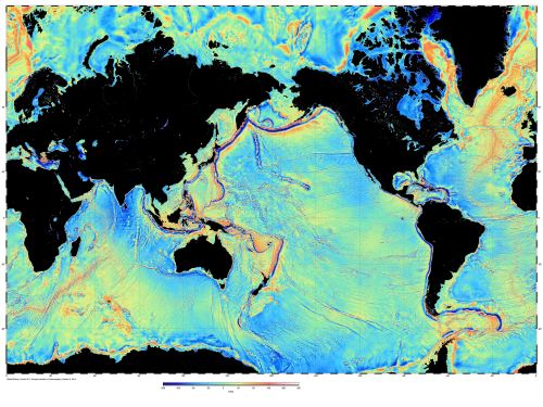
Global gravity over the oceans derived from Jason-1 and Cryosat-2 radar altimetry (credit: Scripps Institution of Oceanography)

There are many ways of processing the data, and so years of fruitful interpretation lie ahead of oceanographers and tectonicians, with more data likely from other suitably equipped satellites: sea-surface height studies are also essential in mapping changing surface currents, variations in water density and salinity, sea-ice thickness, eddies, superswells and changes due to processes linked to El Niño.

Earthquakes and radar interferometry

A friend recently moved to the Napa Valley in California, almost certainly motivated by the vast area given over to the grape and the quality of Napa wines. Shortly after the flit, in the middle of some minor refurbishment, he had quite a shock; a Magnitude 6.0 earthquake at 3:20 a.m. local time on 24 August, the worst in northern California for 25 years. My friend lives only 15 km from the epicentre in South Napa, but his house was undamaged. His confidence in the move remains unshaken, however, as there was no effect on this year’s grape harvest.

The event was monitored by the European Space Agency’s Sentinel-1A high-resolution radar satellite that entered orbit in April 2014. Sentinel revisits any area on the ground every 12 days, has all-weather/day-night imaging capacity, a 250 km-wide image swath with 10 m spatial resolution and is designed to analyse ground movements using interferometry between radar data before and after events. Interferometric radar imaging or InSAR relies on changes in the phase of radar waves between two dates of ‘illumination’ of the ground – radar images normally use only the amplitude of a radar wave, ignoring its phase – and potentially can measure shifts in ground elevation of the order of centimetres.

Interferometric radar image of the area around San Francisco showing the ground movement for the period before and after the
Interferometric Sentinel-1A radar image of the area around San Francisco showing the ground movement for the period before and after the Napa Valley earthquake (NE corner) of 24 August 2014 (credit: ESA)

The image records ground movement in small steps of elevation that are assigned colours, the sequence blue-green-yellow-red-magenta spans a ground shift of about 3 cm. If several of these ‘fringes’ are closely spaced over relatively small areas this is due to significant motions locally. Broad areas with little change in colour have barely moved in the period between the dates of the two images.

The epicentre of the South Napa earthquake clearly shows up at the NE corner of the image, like half a ‘bull’s eye’. A closer look at the enlarged image (click on the image) shows two such features sharply bounded to the west by a line: that coincides with the West Napa Fault.

My friend lives to the west of the faults where the broad areas of colour signify much smaller motions than in the main affected area. He woke and left the building thinking this was a foreshock of a much more destructive event, and had an anxious few days. The United States Geological Survey  estimated that during the main ‘quake 15,000 people experienced severe shaking, 106,000 people felt very strong shaking, 176,000 felt strong shaking, and 738,000 felt moderate shaking. But there was only one fatality and 13 hospitalised casualties.

Remote sensing for fossils

With the growing diversity of data from those parts of the electromagnetic spectrum that pass freely though Earth’s atmosphere, mainly acquired from orbit, an increasing number of attributes of the surface can be mapped remotely. The initial impetus to launch remote sensing satellites in the 1960’s and early 70’s had two strands: to monitor weather conditions and assess vegetation cover with the early metsats, such as TIROS-1, and the first Landsat platform that exploited green plants’ propensity for absorbing visible and largely reflecting near-infrared (NIR) radiation. With the incorporation in the Advanced Spaceborne Thermal Emission and Reflection Radiometer (ASTER) instruments of wavelength regions in which minerals show spectral diversity, in the reflected short-wave infrared (SWIR) and emitted thermal infrared (TIR), remote sensing became a viable and useful tool for geologists. It figures strongly in lithological mapping and also in the detection of minerals related to various kinds of alteration associated with metal mineralisation and the migration of hydrocarbon-related fluids. The more wavebands with narrower coverage of radiation wavelengths, the more likely are the subtle differences in mineral spectra able to be detected and mapped. Yet, apart from one experimental system (Hyperion aboard NASA’s EO-1 orbital platform) our home planet is not as well served by such hyperspectral systems as is Mars, blessed by two which have fuelled the on-going search for past habitable zones on the Red Planet.

The May 2014 issue of Scientific American includes an article on remote sensing that follows what to many might seem an odd direction: how to increase the chance of finding rich fossil deposits (Anemone, R.L. & Emerson, C.W. 2014. Fossil GPS. Scientific American, v. 310(5), p. 34-39). Apart from targeting a particular stratigraphic unit on a geological map, palaeontological collection has generally been a hit-or-miss affair depending on persistence and a keen eye, with quite a lot of luck. Once a productive locality turns up, such as the Cambrian Burgess shale, the dinosaur-rich Cretaceous sandstone of the Red Deer River badlands of southern Alberta in Canada and the hominin sites of Ethiopia’s Afar Depression, palaeontologists often look no further until its potential is exhausted. Robert Anemone and Charles Emerson felt, as may palaeobiologists do, that one fossil ‘hotspot’ is simply not enough, yet balked at the physical effort, time and frustration needed to find more by trekking through their area of interest, the vast Tertiary sedimentary basins of Wyoming, USA. They decided to try an easier tack: using the few known fossil localities as digital ‘training areas’ for a software interrogation of Landsat Enhanced Thematic Mapper data in the hope that fossiliferous spots might be subtly different in their optical properties from those that were barren.

Satellite image of the Wyoming Basin, Wyoming,...
Satellite image of the Wyoming Basin, USA. credit: Wikipedia)

The teeth and bones of early Eocene mammals that had drawn them to Wyoming turn up in sandstone beds of the basins. They are pretty distinctive elements of landscape, forming ridges of outcrop because of their relative resistance to erosion, yet for that very reason present a huge selection of possibilities. Being simple mineralogically they also presented a seemingly daunting uniformity. Anemone and Emerson decided on a purely statistical approach using the six visible, NIR and SWIR bands sensed by Landsat ETM, rather than a spectrally oriented strategy using more sophisticated ASTER data with 14 spectral bands. Their chosen algorithm was that based on an artificial neural network that the fossil rich sandstones would train to recognise patterns present in ETM data recorded over them. This purely empirical approach seems to have worked. Of 31 sites suggested by the algorithm 25 yielded abundant vertebrate fossils. Applied to another of Wyoming’s Tertiary basins it also ‘found’ the three most productive known mammal sites there. So, what is it about the fossil-rich sandstones that sets them apart from those that are more likely to be barren? The authors do not offer an explanation. Perhaps it has something to do with reducing conditions that would help preserve organic material better than would sandstones deposited in an oxidising environment. Iron minerals and thereby colour might be a key factor, oxidised sandstones are generally stained red to orange by Fe-3 oxides and hydroxides, whereas reduced sandstone facies may be grey because of iron in the form of sulfides

Enhanced by Zemanta

An early magma ocean on Mars?

The division of the lunar surface into two petrological domains – ancient anorthositic highlands and younger basaltic maria – spurred the idea, as long ago as the early 1970s, that the early Moon had a deep ocean of magma at the surface, whose cooling caused fractional crystallization. Low density plagioclase feldspar, dominated by high-calcium anorthite and bytownite, floated to the surface to form the lunar anorthosites leaving a more mafic mantle from which the mare basalts formed by partial melting. The key evidence in support of this hypothesis lies in the rare-earth elements of the two terrains. Because plagioclase feldspar has a much stronger affinity to incorporate the element europium (Eu) than the other REEs, the lunar anorthosites are enriched in Eu compared with its related elements. If the highland anorthosites did form by fractional crystallisation the remaining magma that formed the lunar mantle would be depleted in Eu yet enriched in the remaining REE. Although there are no samples of the Moon’s mantle there are plenty of the mare basalts that formed when it partially melted, probably as a result of huge impacts around 3.8 billion years ago. They should have inherited dominant features of mantle geochemistry, and indeed they do show characteristic depletion of Eu.

Lunar Highlands, near Descartes Crater. Collec...
Lunar Highland anorthosite, collected by the crew of Apollo 16. (credit: Wikipedia)

The giant-impact hypothesis for the Earth-Moon system presupposes that such a cataclysm would have left much of the outer Earth in much the same molten condition and destined to fractionate in the same manner. There are geochemical hints from terrestrial rocks that do support such an idea. An important target for exploration of Mars has been to check if a magma ocean also existed early in its history. Of the various missions in recent years only two have the capacity to shed useful light on the issue: the US Mars Reconnaissance Orbiter and Mars Odyssey. Both orbiters carry more sophisticated remote sensing instruments than any circling the Earth. The first has the hyperspectral Compact Reconnaissance Imaging Spectrometer for Mars (CRISM) that senses visible to short-wave infrared (VNIR) radiation, the other deploys  the Thermal Emission Imaging System (THEMIS) that captures different parts of the longer wavelength thermal infrared (TIR) spectrum emitted by surface materials. Both allow spectra of surface materials to be reconstructed and compared with the features of known minerals from the Earth and Moon.

Feldspars are highly reflective for the most part of  the VNIR range but show a shallow, broad absorption feature centred on a wavelength of 1.26 micrometres. Such spectra have been detected using CRISM from parts of the Martian surface in the highlands of its southern hemisphere (Carter, J. & Poulet, F. 2013. Ancient plutonic processes on Mars inferred from the detection of possible anorthositic terrains. Nature Geoscience, v. 6, p. 1008-1012). The authors, from Chile and France, acknowledge that the plagioclase-rich rocks occur only in small patches, unlike the vast tracts on the Moon, and also that on Earth anorthosites are known to have formed by a variety of processes from far smaller magma systems than a veritable ocean of molten rock. Feldspars also show spectral features in the TIR, though not so distinctive, both plagioclase and alkali feldspars being very similar. Moreover, THEMIS deploys sensor for only 10 thermal wavebands, compared with 544 on CRISM.  A team of US remote sensers (Wray, J.J. and 8 others 2013. Prolonged magmatic activity on Mars inferred from the detection of felsic rocks. Nature Geoscience, v. 6, p. 1013-1017) used both CRISM and THEMIS data. While noting resemblances to lunar anorthosites, they adopt a more cautious approach to the spectra and prefer the broad, ‘sack’ term ‘felsic rocks’. It seemed possible from their work that feldspar-rich magmas may have formed by partial melting of common andesitic crust noted from the Martian surface: high spatial resolution images of the occurrences bear some resemblance to outcrops of granitic rocks in arid environments on Earth. That is, there may be highly evolved rocks akin to terrestrial continental crust.

The interesting spectral observations on Mars can only be validated by actual rock samples. While rovers still operating on the Martian surface are well able to produce geochemical data that would petrologically characterise most rocks that they encounter, none of them is in a terrain suitable for resolving this particular issue. Yet, coincidentally, a meteorite found in West Africa shows hallmarks of having been blasted from the surface of Mars and sheds useful light on various hypotheses about the Martian crust http://earth-pages.co.uk/2013/11/21/a-glimpse-of-early-martian-crust/. It is a breccia that may represent the soil or regolith that accumulated from early impacts that shattered and melted surface materials, and it is extremely old: zircons yielded an age of 4428 Ma. The clasts set in a fine matrix consist of a variety of igneous rocks, none of which are anorthosites. Some are coarse grained, plutonic rocks containing both alkali feldspars and plagioclase, which match terrestrial monzonites; broadly speaking members of the granite family. Having formed from the ejecta of large impacts, such regolith materials represent the breadth of compositions across the planet and extending deep into its crust. This one suggests that anorthosites may have been rare on early Mars.

The Grand Greenland Canyon

One of the properties of radar is that it can pass through hundreds of metres of ice to be scattered by the bedrock beneath and return to the surface with sufficient remaining power to allow measurement of ice depth from the time between transmission of a pulse and that when the scattered energy returns to the antenna. Liquid water simply absorbs the radar energy preventing any return from the subsurface. As far as rocks and soils are concerned, any water in them and the structure of minerals from which they are composed limit penetration and energy return to at most only a few metres. While radar images that result from scattering by the Earth’s solid surface are highly informative about landforms and variations in the surface’s small-scale texture, outside of seismic reflection profiling, only ice-penetrating radar (IPR) approaches the ‘holy grail’ of mapping what lies beneath the surface in 3-D. Unlike seismic surveys it can be achieved from aircraft and is far cheaper to conduct.

English: Topographic map of Greenland bedrock,...
Greenland’s topography without the ice sheet. (Photo credit: Wikipedia)

It was IPR that revealed the scattering of large lakes at the base of the Antarctic ice cap, but a survey of Greenland has revealed something even more astonishing: major drainage systems. These include a vast canyon that meanders beneath the thickest part of the ice towards the island’s north coast (Bamber, J.L. et al. 2013. Palaeofluvial mega-canyon beneath the central Greenland ice sheet. Science, v. 341, p. 997-999). At 750 km long and a maximum depth of 800 m it is comparable with active canyon systems along the Colorado and Nile rivers in the western US and Ethiopia respectively. A less-well publicised feature is ancient leaf-shaped system of buried valleys further south that emerges in a great embayment on West Greenland’s coast near Uummannaq, which may be the catchment of another former river system. In fact much of the data that revealed what appears to be pre-glacial topography dates back to the 1970s, though most was acquired since 2000. The coverage by flight lines varies a great deal, and as more flights are conducted, yet more detail will emerge.

The British, Canadian and Italian discoverers consider that glacial meltwater sinking to the base of the ice cap continues to follow the canyon, perhaps lubricating ice movement. The flatter topography beneath the Antarctic ice cap is not so easy to drain, which probably accounts for the many sub-glacial lakes there whereas none of any significance have been detected in Greenland. The earliest time when Greenland became ice-bound was about 5 Ma ago, so that is the minimum age for the river erosion that carved the canyon

On-line global geological maps

This item about the OneGeology map portal can now be read at Earth-logs in the Remote Sensing archive for 2013

OneGeology1
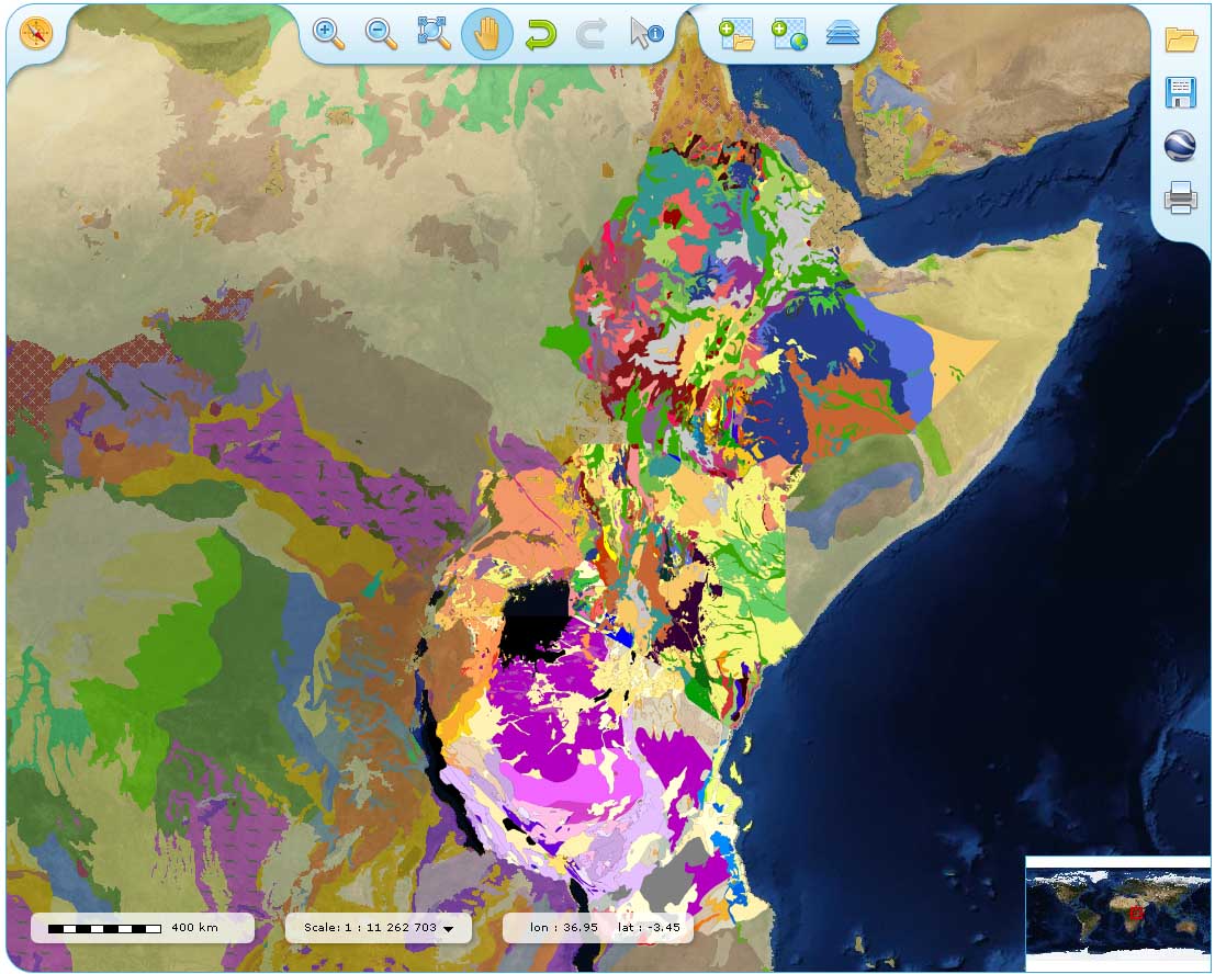
Small-scale extract from the OneGeology portal with 1:2 million maps for Ethiopia, Kenya, Tanzania and Uganda, and at 1:10 million covering surrounding areas (credit:OneGeology portal)


More wet minerals on Mars

A remote-sensing geologist who focuses on terrestrial matters would likely grind their teeth on seeing papers that use far better data captured from the Martian or lunar surface than are ever likely to be available from the bulk of Earth’s land surface over the next decade at least. Mine are even closer to the gums after reading about hyperspectral data from Mars with high spatial resolution (~20 m), used to locate rocks altered by water on Mars (Carter, J. et al. 2010. Detection of hydrated silicates in crustal outcrops in the northern plains of Mars. Science, v. 328, p. 11682-1686). And, of course, there is no vegetation and not much of an atmosphere to cryptify spectral features of minerals: if there is enough of a mineral exposed to show up, the Compact Reconnaissance Imaging Spectrometer for Mars (CRISM) carried by NASA’s Mars Reconnaissance Orbiter will spot it. If the mineral has unique features in its spectrum, and most of the hydrated silicates do, it can be classified nicely. Less spatially sharp hyperspectral data from the Observatoire pour la Minéralogie, l’Eau, les Glaces et l’Activité (OMEGA) carried by ESA’s Mars Express is equally discriminating for larger patches.

The two instruments have shown up hundreds of small outcrops of minerals in the southern hemisphere that formed by reactions between the dominantly anhydrous minerals of Mars’s dominantly igneous crust and water. They record an early phase when liquid water was available at the surface. The question is, are they merely a thin veneer? As a check, John Carter (did bearing the same name as Edgar Rice Burroughs’ hero in his Mars novels encourage his fascination with the Red Planet?) of the University of Paris and colleagues used OMEGA and CRISM data to look at deep crust exhumed in several of Mars’s northern hemisphere craters. Clay minerals, chlorite and prehnite do show up clearly, and the hydration reactions must therefore have penetrated up to a kilometre into the crust. The same suite of minerals occur in the southern hemisphere, so during this early wet episode water was available far and wide across the Martian surface. Minerals like prehnite and chlorite are most familiar as products of low-grade metamorphism, which presents a puzzle. Maybe they formed as a result of the temperatures and pressure generated by the impacts themselves. But if that were the case they would be expected to pervade all the excavated rock, whereas they occur in distinct patches next to pristine, highly reactive olivine-rich rocks. One absentee mineral is serpentine that would definitely have formed by the reaction of water with olivine during impacts. So it looks like water pervaded the whole Martian crust down to maybe a kilometre, then this ‘weathered’ layer was blanketed much later by a thick volcanic layer which has been removed in some places by impact excavation.

• Tectonics
Underpinnings of Mediterranean tectonics
The region of the Mediterranean Sea, especially in the Aegean area, has among the most complex active tectonics on Earth. Both the African and Eurasian plates are now barely moving. The basic shaping of the region stems from Africa’s protracted collision with Europe since 40 Ma that resulted in the closure of the Mesozoic Tethys seaway and jumbled both its sedimentary fill and the continental lithosphere that lay on either side of the collision zone. But if surface motion has largely stopped, why is the Mediterranean region so tectonically active? It now seems as though it links to flow in the mantle beneath (Facenna, C. & Becker, T.W. 2010. Shaping mobile belts by small-scale convection. Nature, v. 465, p. 602-605). A mix of GPS tracking of surface motions, evaluation of surface uplift and subsidence, and analysis of seismic tomography of the mantle. Vertical motion of the mantle is most pronounced at shallow mantle depth (250 km), suggesting vigorous convection in quite small cells. The relations to tectonics are complex, but they are interlinked. For instance subducting slabs interfere with shallow mantle flow so that compensating upwellings result, and in turn help drive subduction and volcanism, as in Italy. Overall, the lithospheric motion, from GPS tracking, has a distinct vortex-like pattern in the eastern Mediterranean and Middle East, which can be modelled from the underlying mantle flow.

Geochemical prospecting on Mars

Since its atmosphere is so thin, there are things you can achieve from orbit around Mars that would be unthinkable for the Earth. One is imagery free of atmospheric shimmer or scattering, another is analysing gamma rays emitted by Martian rocks using a gamma-ray spectrometer (GRS), as carried by Mars Odyssey. Two processes produce the gamma rays: the decay of long-lived naturally-occurring radiogenic isotopes of potassium, uranium and thorium with their daughter isotopes, and by the interactions of high-energy cosmic-ray particles with other elements in surface materials. Again, with little atmosphere the Martian surface is heavily bombarded by cosmic rays. Using far larger gamma-ray detecting crystals carried on low-flying aircraft it is possible to remotely sense K, U and Th concentrations at the Earth’s surface. To get data on other terrestrial elements from far off would involve unsociable irradiation of the surface by artificial means.

Results from the Mars Odyssey GRS are somewhat blurred as the analysed radiation comes from 0.5º x 0.5º sampling ‘bins’ and is then filtered to a level of 5º x 5º (~ 25 x 25 km) (Taylor G.J. et al. 2010. Mapping Mars geochemically. Geology, v. 38, p. 183-186). So, the approach cannot match geological maps made by interpretation of high resolution images of reflected or thermal radiation. However, as well as K, U and Th estimates, the data cover Fe, Si, Ca, Cl and H2O: sufficient to crudely distinguish mafic and felsic igneous rocks and to detect any regional hydrothermal or groundwater alteration. The authors claim that the GRS separates  much of the Equatorial region of Mars into six kinds of geochemical province, all of roughly basaltic composition. With an estimated SiO2 range from 46.7 to 49.8% that doesn’t promise much by way of fractionation on the scale of terrestrial magmagenesis; i.e. there are no significant intermediate or felsic igneous rocks. A CaO range of 7.5 to 11.4 does indicate varying plagioclase feldspar content, but no anorthosites, unlike the Moon. The greatest variation is in K and Th content, but that does not match the much larger ranges in terrestrial basalts. The geochemical provinces do not match even a simplified photogeological map of the planet, and it seems quite likely that such variation as there is could have resulted from slight weathering and movement of dust and sand. Will a single returned sample of Mars basalt be all that is needed to characterise the Red Planet? More to the point, how does the estimated chemistry match that of purported Martian meteorites, or for that matter the analyses performed on the surface by the Martian rovers Spirit and Opportunity and by the earlier Mars Pathfinder? There is no comment…but Mars Pathfinder surface analyses revealed andesitic rocks at its landing site with up to 55% SiO2.

Micro-gravity data chart shrinking ice caps

The NASA and German Aerospace Centre Gravity Recovery and Climate Experiment (GRACE) launched in 2002 aims to measure variations over time in the Earth’s gravity field by gauging tiny changes in distance between two satellites using radar. Briefly, mass in the Earth tugs first on the leading satellite and then on the one trailing it, so if mass distribution stays constant so does the separation between the craft. If mass below a point on the Earth’s surface does change, GRACE detects this from a change in separation between the two craft. Between April 2002 and February 2009, monthly measurements over Greenland and Antarctica reveal losses in the amount of ice, and the rate at which the ice caps are shrinking is accelerating (Velicogna, I. 2009. Increasing rates of ice mass loss from the Greenland and Antarctic ice sheets revealed by GRACE. Geophysical Research Letters, v. 36, L19503 doi:10.1029/2009GL040222). Isabella Velicogna of NASA/JPL shows that the Greenland ice cap (total mass~3 x 10¹⁵ t) lost 1.37 x 10¹¹ t a-1 in 2002–3, rising to 2.86 x 10¹¹ t a-1 in 2007–9 , the loss is accelerating at 3.0 ± 1.1 x 10¹⁰ t a-2). The ten times more massive Antarctic ice cap lost 1.04 x 10¹¹ t a-1 in 2002–6 rising to 2.46 x 10¹¹ t a-1 in 2006–9, giving an acceleration of 2.6 ± 1.4 x 10¹⁰ t a-2. Proportionate to size the Greenland ice cap is dwindling faster than Antarctica, but at these rates it still has 10 thousand years before it disappears.

Wow! Columnar joints found in Martian lava flow…

From time to time I wear my spleen on my sleeve over issues of scientific priority. Orbiting Mars are imaging devices whose data, if they were of the Earth’s surface, would cost geoscientists the proverbial arm and a leg.  ‘Astrogeologists’ get those from Mars for nothing. The latest result explains why I get annoyed; and I hope many others do as well (Milazzo, M.P. and a great many others 2009. Discovery of columnar jointing on Mars. Geology, v. 37, p. 171-174). The High Resolution Imaging Science Experiment (HiRISE) aboard the Mars Reconnaissance Orbiter, can resolve pixels 30 cm across (about the same as the best, classified military data of Earth from spy satellites). It has stereoscopic capacity capable of producing not only stunningly informative 3-D visualisations but also topographic elevation data sufficiently precise that they could be used ‘at home’ for large-scale civil engineering, for instance routing water pipelines. The US Department of Defence vetoes access by scientists to near-global SRTM DEMs with even a 30 m resolution, the degraded 90 m version being freely available. Sub-metre DEMs can be produced from aircraft for the Earth’s surface, but at very high cost.

The paper reports one of the most common features exhibited by thick lava flows and other tabular bodies of igneous rock that cooled slowly. Visit the Giant’s Causeway in Antrim to see columnar joints, and put your child on one for scale. In fact there are thousands of such sights on Earth, and any planet that has a volcanic history will have columnar joints. Similar quality data is awaited from the Moon, and you can bet your intimate garments that some bright spark will report much the same. Meanwhile, there are over a billion people drinking hazardous water when geologists armed with data this good – and the inclination – could find safe supplies in the rocks beneath them.

Entire Landsat archive now accessible by all, free of cost

May 2008 saw probably the most significant announcement for geologists of this century (The Landsat Science Team 2008. Free access to Landsat imagery. Science, v.  320, p. 1011; and see landsat.usgs.gov/images/squares/USGS_Landsat_Imagery_Release.pdf). Given a broadband internet connection, it will soon be possible to download Landsat data (MSS, TM and ETM+) covering any area on Earth free of charge from the US Geological Survey, provided it occurs among the >2 million scenes archived by their EROS Data Center. This act of open-handed generosity by the USGS marks a key step in revolutionising the activities of geologists of the Third World, especially those in Africa; the least well-mapped continent. Landsat data and those from the Japanese-US ASTER instrument aboard the Terra satellite offer huge potential for mapping rocks and soils, especially in dry lands, at scales of up to 1:50 000. Africans need to know about their physical resources, especially water, instead of well-heeled mining, petroleum and consulting companies from rich countries, who have more or less monopolised (and sometimes eked out) knowledge of the continent’s riches. Now they can begin to find out for themselves.

Satnavs useful to hydrogeologists as well as white-van drivers

Microwave radiation emitted by radar remote sensing systems does not merely produce useful images of the Earth when all else fails because of cloud cover. They interact with the surface in such a way that their characteristics change, specifically when the moisture content of surface materials such as soil varies. This phenomenon has spurred development of satellite-borne estimation of soil moisture. But since the launch of constellations of satellites aimed at precise navigation, such as the well-known US Global Positioning System (GPS) and Europe’s Galileo system, everywhere on the Earth is continually bathed in weak microwaves. Researchers at the University of Colorado, Boulder have done a test of the concept using a single GPS receiver recording continuously at one site in Tashkent, Uzbekistan (Larson, K.M. et al. 2008. Using GPS multipath to measure soil moisture fluctuations: initial results. GPS Solutions, v. 12, p. 173-177).

Multipath signals are received when an electromagnetic signal arrives at an antenna, not along a direct path from its source, but indirectly due to reflection of the signal by an object or surface near the antenna. Multipath contaminates all GPS measurements, leading to small positional errors, because the receiver locks onto a signal that mixes the direct and reflected signal. It is difficult to isolate the effects of multipath in GPS carrier phase signals. However, the signal-to-noise ratio (SNR) data computed by a GPS receiver are also affected by multipath and provide an easier route to quantifying multipath effects.  In fact the authors found that the amplitude of the SNR varies over time and correlates well with variations in local soil moisture following rainy and dry episodes. Although a first test of concept, the results are sufficiently encouraging that specialist GPS receivers may be developed that allow both precise positioning and accurate measurements of soil moisture – what may become a must for hydrogeologists, especially in arid and semi-arid terrains.

Desert varnish

Just as vultures are annoyed by glass eyes, so geologists who use remote sensing detest vegetation cover. But the spectral blanket thrown over geology by grass and other plants is not the only irritation and one occurs where least expected. Arid terrain usually pays the best dividends in remote geological mapping, because the spectral properties of rocks and their constituent minerals emerge in reflected and emitted radiation  and bear close relationships to those determined in laboratories. Images captured from orbit that use carefully chosen wavebands are often stunningly informative in deserts. The bugbear is desert varnish, an often shiny black coating that completely masks what lies beneath, be it basalt, granite, sandstone or carbonate, even in the field. Generally it is no more than a millimetre thick, and often far thinner. Close examination often shows a minutely botryoidal texture and parallel laminae in cross section, very like a tiny stromatolite. Basically, desert varnish is such a biofilm deposit, and the responsible organisms are cyanobacteria, as in stromatolites, but exceptionally sturdy ones. However, the bulk of the material is inorganic, and it is spectrally featureless, hence the problem in remote sensing.

Widespread as it is in arid environments, desert varnish has not been deemed an appropriate subject of study, so any information is welcome (Garvie, L.A.J. et al. 2008. Nanometer-scale complexity, growth and diagenesis in desert varnish. Geology, v. 36, p. 215-218). Hailing from Arizona University, the authors are well placed. Their approach is no so much directed at organic aspects, which is a shame, but at the geochemistry of this annoying gunk. As previously known, they show the dominance of manganese phases, but mixed in with very fine-grained quartz, clays and iron oxy-hydroxides. The varnish seems to contain a wind-blown component, but the manganese and probably the iron is derived in some other way, having grain sizes less than 100 nanometres. Iron and manganese minerals dominate the fine laminae, and at very high electron microscope resolutions their grains show yet finer structure at 1 nm scale. The authors ascribe the cyclical structures and mineralogy to repeated wetting and drying, with leaching and oxidation of Fe and Mn. Both iron and manganese are multi-valent, Mn more so than Fe. For both to be leached, i.e. drawn into solution as Fe2+ and Mn2+ ions, requires strongly reducing conditions, and then oxidation to precipitate Fe3+ and Mn4+ or Mn7+ minerals. At this minute scale, whatever the source of the Fe and Mn, a biological influence seems crucial.

Renewed interest in desert varnish seems to be connected with Mars – the study was partly financed by NASA. Yet, none of the Martian remote sensing studies report annoyance with huge tracts blacked out by manganese minerals. Such surface alteration that has been analysed by the Mars Rovers proved to be iron-enriched with little significant manganese enrichment. If desert varnish is biogenically mediated, then its occurrence on Mars would be cause for excitement bordering on hysteria. The cyanobacteria in terrestrial varnishes are tough, and may date back into Precambrian times as the first colonisers of dry land. As yet, there have been no attempts to examine their genetic affinities.

Detecting, mapping and understanding ancient soils

A recent paper provides a clear guide and a new means of addressing one of geoscience’s great puzzles (Andrew Deller, M.E. 2006. Facies discrimination in laterites using Landsat Thematic Mapper, ASTER and ALI data — examples from Eritrea and Arabia. International Journal of Remote Sensing, v. 27, p. 2389–2409). During the early Cenozoic, and perhaps before that, huge areas of the exposed continental surface were subject to a hot, humid climate. Intense chemical weathering broke down every conceivable rock type to a few stable minerals. The resulting residual soils were preserved over vast areas of Africa, South America, India and Australia to form laterites, which M.E. Andrews Deller at the Open University UK points out are distinctly zoned [avoids repeat of layered] mineralogically and stunningly layered in colour. No one can fail to see laterites where they are exposed, if they know what to look for, but few geologists have set out to understand them properly. Andrews Deller documents in detail where these unique rocks occur, highlighting the importance of laterites as a resource; the frightening hazards that they pose to people throughout laterite-mantled Africa, and their relevance to the history of erosion and intraplate deformation.

The central theme of Andrews Deller’s paper is the essential first step of mapping laterites and discriminating their facies. This rests on their mineralogical simplicity, and the unique and distinct spectral properties of those constituent minerals. The author matches these to the spectral coverage of freely available remote sensing data — Landsat TM, ASTER and ALI — each of which offers nuances to be exploited in uniquely discriminating the different laterite horizons. Rather than setting out to ‘unveil’ sophisticated new methods of computer analysis (to which few people in laterite-encrusted areas would have access), Andrews Deller explores the simplest, most revealing approaches to a previously overlooked challenge: laterite facies have never been discriminated and mapped before using remote sensing. The results in this well-illustrated paper are stunning, and any geologist (and probably many lay people) can understand what the figures show and the importance of mapping laterites, thanks to careful discussion. The result is a paper that combines interest, novelty and usefulness.

Detecting and mapping ancient soils

During the early Cenozoic, and perhaps before that, huge areas of the exposed continental surface were subject to hot humid climatic conditions. That broke down every conceivable rock type to a few simple minerals that were both stable and insoluble. Such intense weathering possibly affected 30% of the land area during those ‘hothouse’ times. Where the surface was flat, the resulting residual soils were preserved to form laterites, strongly layered mineralogically. Since one of the common components is bright-red hematite, and its brown hydrous equivalent goethite, and another is brilliant white kaolinite, laterites are also stunningly layered in colour from white iron-poor clays at their base through an middle mottled yellow, orange, pink and white zone, to brick-red iron-rich ferricrete at the top of the sequence. No-one can fail to see laterites where they are exposed, but few geologists have set out to understand them. A recent paper provides a clear guide to begin that work on a grand scale, and also to chart where their unique properties and socio-economic pros and cons can be developed or avoided respectively (Andrew Deller, M.E. 2006. Facies discrimination in laterites using Landsat Thematic Mapper, ASTER and ALI data—examples from Eritrea and Arabia. International Journal of Remote Sensing, v. 27, p. 2389–2409).

The key to the long and complex chemical and mineralogical evolution of laterites lies in the different layers or facies in these palaeosols. Because they are thin and once present over vast areas of Africa, South America, India and Australia, their presence or absence today is a guide to the history of erosion and intraplate deformation after they formed. Each facies has very different chemical and physical properties, some advantageous, and some decidedly a threat of some kind, recognised and well documented by M.E. Andrews Deller of the British Open University. For instance, the clay zone is a lubricant that can encourage landslides of great thicknesses of overlying rock, yet is a potential resource — it is China Clay. Hard and porous ferricrete, containing both iron minerals and clays, makes it a cheap source of bricks and even road aggregate. But hematite can pose a frightening risk. Its open structure soaks up dissolved ions, including infamously those of arsenic, which lateritisation can set in motion from the rocks on which it develops. Hematite dissolves under reducing conditions, and should those develop on old laterites arsenic might be liberated to groundwater. Another associated compound that laterites can release is magnesium sulfate (Epsom Salts), an natural emetic but also a potential remedy for eclampsia that threatens mothers and their babies throughout laterite-mantled Africa.

Andrews Deller’s paper is a mine of laterite-related information, yet its central theme is the essential first step of mapping them and discriminating their facies. Her starting point is their mineralogical simplicity, and the unique and distinct spectral properties of those constituent minerals. She matches these to the spectral coverage of freely available remote sensing data — Landsat TM, ASTER and ALI — each of which offers nuances to be exploited in uniquely discriminating the zones. Rather than setting out to ‘unveil’ sophisticated new methods of computer analysis (to which few in laterite-encrusted areas would have access), she chose the simplest useful approaches to a previously overlooked challenge: laterite facies have never been discriminated and mapped before. The results in this well-illustrated paper are stunning, and any geologist, and quite likely many lay people can understand what they show, thanks to careful discussion. The result is a paper that combines interest, novelty and usefulness. The last is the best aspect: geologists can learn from the paper how confidently to make highly informative maps cheaply and quickly.

ASTER data and earthquakes

NASA’s Jet Propulsion Laboratory in Pasadena, California is a huge engine of across-the-board innovation. In my field, remotely sensed geology, everyone pounces eagerly on publications by its scientists because they are bound to push techniques and applications forwards, often in surprising contexts, such as archaeology from space. One such nugget is about to be published (probably this month) in the premier geoscience journal EPSL (Avouac, P. et al. 2006. The 2005, Mw 7.6 Kashmir earthquake: Sub-pixel correlation of ASTER images and seismic waveforms analysis. Earth and Planetary Science Letters, in press doi:10.106/j.epsl.2006.06.025) and amply justifies my impatient preview here. It offers great potential for monitoring the effects of natural hazards that involve mass motion using free (for bona fide researchers and, hopefully, humanitarian organizations) satellite image data.

Jean-Phillipe Avouac and colleagues at JPL applied a well-tried approach in remote sensing — comparison of images captured on different dates—in trying to assess the extent and magnitude of ground motion involved in the 8 October 2005 Kashmir earthquake that claimed at least 80 thousand lives. But theirs is a before-and-after study with a revolutionary new slant. ASTER data from the joint US-Japanese Terra satellite resolves the ground with a resolution as sharp as 15 m, in several wavebands of EM radiation. In their own right, these bands contain huge amounts of information about vegetation, rocks and soils, and many other environmental attributes. Particularly with vegetation, comparing data from different years or seasons soon shows up changes and clues as to why they occurred. But ASTER has another potential view to offer. Two of its sensors, one pointing vertically downwards, the other obliquely back along its ground track, constitute a stereopair. They can be viewed together to give dramatic 3-D visualizations of terrain. With the appropriate software, the parallax difference between the location of each point on the ground in the two images produces a map of terrain elevation. The novelty and potential in Avouac et al. is to combine ASTER data from two instants in time to find places that have shifted in position in the meantime. So that they match geographically, they used stereo-derived terrain elevation to remove geometric distortions caused by viewing rugged relief with effectively a wide-angle camera. The key to extracting deformation parameters is applying shape-detection software to images from before and after an event, and then finding the magnitude and direction of the differences between landform shapes to chart movement. The 15 m resolution poses a limit, but the sophistication of the algorithms enables shifts of the order of less than a metre to be detected at a coarse resolution of 150 m. But that is quite sufficient to show what happened in Kashmir along the entire length of fault movement in 2005. Applied to commercially available stereo data (up to 0.65 m resolution) the results would be awesome.

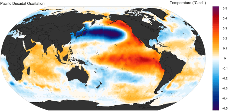
Mineral mapping and the history of Mars’ rocks and water

The principal mineral and rock mapping tool for Mars is the Observatoire pour la Minéralogie, l’Eau, les Glaces, at l’Activité. OMEGA is every remote sensing geologist’s dream machine, because its coverage of the short-wave end of electromagnetic radiation by 350 narrow bands can match spectra reflected from rocks and soils with those measured under laboratory conditions for several hundred important minerals. For over 18 months it has been steadily building up mineralogical maps of the Martian surface in a series of narrow swathes would round the planet in the manner of wool in a ball (see Mineral maps of Mars in April 2005 issue of EPN for early results). The 90% complete data, combined with dating of surface regions from crater counts and other means of stratigraphic analysis, is beginning to chart the history of the Martian surface in familiar terms of geology and the effects of water (Bibrin, J-P, and a great many others in the OMEGA team 2006. Global mineralogical and aqueous Mars history derived from OMEGA/Mars Express data. Science, v. 312, p. 400-404).

An interesting correlation is emerging. Where Mars’s surface is dominated by large amounts of pyroxene – the stratigraphically older regions of heavily cratered volcanic rocks – there is evidence of hydrated clay minerals (products of non-acid water alteration) and sulfates (formed by acid, hydrous alteration). The younger, brighter regions, which probably formed by surface processes after about 3.5 Ga, are dominated by anhydrous iron(III) oxides that give Mars its overall red colour. Although on Earth this hematite commonly forms by dehydration of iron(III) hydroxide or goethite, there is no sign of relic goethite on Mars. The authors attribute the red-staining hematite to direct oxidation of iron-rich silicates, without the role of water. It seems that in terms of surface processes, water played a role in the very earliest weathering to form clays. For a while conditions became acidic by the oxidative breakdown of igneous sulfides, thereby encouraging the formation of sulfate encrustations and sediments. This ‘wet’ phase may well have involved water vapour emanating from early, huge volcanoes. Once global volcanism became extinguished the supply of water was shut off, and since 3.5 Ga the planet has been hyper-arid. Hydrated minerals above the 5% level are not common on Mars, and if they did in fact encourage some life forms to emerge, the search for them can be finely focused by the OMEGA results.

State of the art seismic imaging

For many decades the primary tool of petroleum exploration has been reflection seismic surveying. As oil has become harder to find, industry has hugely improved means of processing seismic waves that return to detectors and expanded data gathering as a means of showing subtle structures and sedimentological detail.  From individual seismic sections up to the 1970s, seismic surveys have moved towards multiple lines with ever-decreasing spacing as a means of producing 3-dimensional subsurface maps. Until recently the results of 3-D seismics have been glimpsed only rarely by the academic community, but once their commercial usefulness has been exploited they are increasingly becoming accessible.  Richard Davies of the 3DLab at the University of Cardiff, UK and Henry Posamentier of Anadarko Canada provide an exquisite overview of the possibilities for research in the October 2005 issue of GSA Today (Davies, R.J. & Posamentier, H.W. 2005.  Geologic processes in sedimentary basins inferred from three-dimensional seismic imaging. GSA Today, v. 15(10), p. 4-9).  They show examples of derivatives from 3-D seismics, produced by a variety of image-processing techniques as well as the basic seismic processing, which demonstrate the depth to which these data can be interrogated.  Featured are an example of meandering Pleistocene channels beneath the Gulf of Mexico, structures produced by sediment compaction between the Shetland and Faeroe islands in the North Atlantic, and the shapes taken by basaltic sills as they flowed into place.  The graphics are wonderful, and would certainly tempt an IT-literate researcher.  However, no funding agency could afford to commission such revealing surveys, and the geoscience community will always rely on the activities and generosity of the petroleum industry to enter this awesome world.  Some might think of midnight meetings at lonely crossroads or an armful of long-handled spoons.  Yet the potential results far transcend the kind of information one might extract from exposed geology.

Mars: the best may yet be to come

The US and ESA satellites orbiting Mars have so far deployed remote sensing instruments that detect visible to thermal infrared radiation from the planet’s surface.  Ultimately the energy involved is from the Sun: these are passive instruments.  Engrossing as they are, images from these sensors reveal only details of surface mineralogy and the Martian topography.  So far, virtually nothing is known about what lies buried beneath it, apart from inferences about ground ice.  The ESA Mars Express has one last imaging trick up its sleeve, which uses energy generated on board and beamed obliquely down to the surface.  This is the Mars Advanced Radar for Subsurface and Ionospheric Sounding (MARSIS).  Radar remote sensing on Earth generally uses high-frequency microwaves in the wavelength range from 0.01 to 0.1 metres, and the images produced show how much energy is scattered by surfaces of varying roughness, to be received by antennae deployed from an aircraft or satellite.  The longer the wavelength the greater the height of small-scale surface irregularities that cause scattering and therefore a received signal.  Smooth perfectly surfaces reflect all the energy away from the antennae, like a mirror, so no energy returns to be sensed.  How microwaves interact with the Earth’s surface depends on the electrical properties of the materials.  Good electrical conductors, such as metals and liquid water are extremely efficient reflectors, whereas minerals are poor conductors and tend to absorb microwaves to some extent.  If soils are extremely dry, with less than 1% moisture content, as in some deserts, some of the absorbed energy is scattered by materials below the surface and images show subsurface features.  This lies behind the principle of ground penetrating radar, but since many soils are damp, only radar waves generated at the surface give good signals in most areas, to be exploited by civil engineers and archaeologists.  Ice is very different from liquid water, being so poorly conductive that it is almost transparent to microwaves.  Consequently it has proved possible to sound the depth of glaciers and ice sheets using ground penetrating radar deployed from aircraft.  The depth of penetration, and of course that involves energy returning to the surface in order to get a signal, is governed by the radar wavelength.  For instance, unknown former courses of the River Nile’s tributaries have been detected by 0.25 m radar waves beneath the hyperarid eastern Sahara through about 3 metres of dry sand.

MARSIS can transmit microwaves with 4 wavelengths 170 , 100 , 80  and 60 m.  Given rocks and soils free of liquid water, which comprise most of Mars’s surface, or ice, it can penetrate as deep as almost 5 km.  The multi-wavelength arrangement can also potentially discriminate water ice from rock and soil.  A great deal of speculation and some evidence suggest that parts of Mars may be underlain by permafrost, that is melted only under unusual conditions, such as after meteorite impacts.  There are also suggestions that glaciogenic-like landforms may still be underlain by ice, and bizarrely that there are frozen seas (see The triumph of the old on Mars in April 2005 EPN).  MARSIS may well throw Mars investigations into a turmoil, but maybe not.  The delay in sparking it up has been caused by fears that deploying its antennae might damage the whole spacecraft, and the first attempt seems to have got stuck.  It’s other drawback is limited power so that horizontal resolution will be between 5 to 10 km and vertically only 100 m, so results may be so blurred as to be inconclusive.  NASA plans a similar device aboard its Mars Reconnaissance Orbiter (launch date August 2005).  The Shallow Subsurface Radar (SHARAD) will use microwaves with 12 to 20 m wavelengths that give penetration to 1 km, but horizontal and vertical resolutions of 300 and 15 metres.

See: Reichhardt, T. 2005.  Going underground.  Nature, v. 435, p. 266-267.