Is there water in the Earth’s core?

Understandably, the nature of what lies at the centre of the Earth is as much the subject of speculation as tangible evidence. That there must be something very dense within the planet emerged once the Earth’s bulk density was calculated. Because a high proportion of meteorites are dominated by an alloy of the metals iron and nickel, geoscientists adopted that combination as plausible core material. Study of the arrival times around the globe of seismic waves from earthquakes then revealed the actual size of the Earth’s core. Iron-nickel alloy fitted the bill quite nicely. It also fits geochemical evidence, such as the crust and mantle’s depletion in some trace elements that theoretically have an affinity for iron. The fact that seismology showed also that the outer core was molten and able to flow, together with metals’ high electrical conductivity, gave rise to the current concept of the geomagnetic field being generated by a dynamo effect in the core. However the density of Fe-Ni is not ‘quite right’ because the core is somewhat lighter than predicted for the pure alloy under stupendous pressure: it must contain a substantial amount – up to 13% – of lower density materials.  Silicon, sulfur and oxygen have been suggested as candidates, with evidence from a variety of minor minerals in metallic meteorites.

A recent model for core formation (credit Crystal Y. Shi et al 2013; DOI: 10.1038/NGEO1956 Fig. 5)

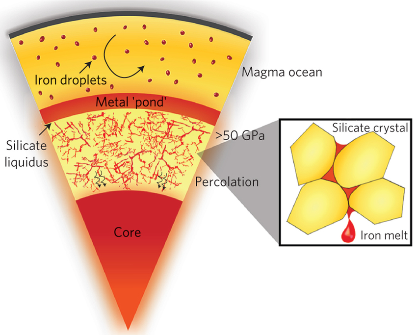
The world is currently awash with models that attempt to throw light on the course of the Covid-19 pandemic. Many are based on highly uncertain data, leading to suggestions by some people that they have become tools for political elites and a means of helping ambitious scientists into the limelight: a sort of fuel for hubris. In the midst of this unprecedented turmoil there has appeared a suggestion (from modelling) that the core also contains abundant hydrogen (Li, Y. et al. 2020. The Earth’s core as a reservoir of water. Nature Geoscience, v. 13, published online; DOI: 10.1038/s41561-020-0578-1). Yunguo Li and colleagues, from University College London, the Chinese Academy of Science and the University of Oslo, explore the idea that the dominant hydrogen of the pre-planetary Solar nebula, which accreted to form the Earth, may have joined iron during core formation. This had been predicted from the thermodynamics of chemical reactions between water and iron. The team takes this further through the geochemical theory that elements and compounds tend to enter other materials preferentially. For example, during partial melting of the crust alkali metals (Na, K etc) are more likely to enter the granitic melt than to remain in the solid residue. Li et al. have used thermodynamics to predict the partitioning of hydrogen between iron and silicate melts under the very high temperature and pressure conditions at the boundary between the core and mantle.

Their calculations suggest that hydrogen then behaves in much the same manner as, say gold and platinum: it becomes ‘iron-loving’ or siderophile and prefers the molten core, as would H2O. The amount that gets in depends on the water content of the molten silicate that eventually becomes the mantle. If the water now making up Earth’s ocean was ‘degassed’ from the mantle during core formation then the original silicate melt would have been ‘wetter’ than it is now. The implication of such early degassing is that the core may contain 5 ‘oceans worth’ of water! The alternative scenario for Earth’s becoming a watery world is the later accretion of, for instance, cometary material. In that case, the early core would have been drier. Yet, the continual subduction of hydrated oceanic lithosphere into the deep mantle during billions of years of plate tectonics would steadily have added water to the core, in the form of iron oxides and hydrogen. So, the core might, in either case, contain several ‘oceans’ of the components of water. One line of indirect evidence is the deficiency in Earth’s actual water of the heavier isotope of hydrogen (deuterium) relative to the D/H ratio of chondritic meteorites. Theory suggests that D has slightly more affinity for joining iron than does H. Substantial water in the core does help explain the core’s apparent low density, but that notion requires as much faith as politicians seem to have in ‘following the Science’ during the current pandemic …

Arsenic hazard on a global scale

I have been following the harrowing story of how arsenic gets into domestic water supplies for 20 years (see: Earth-logs Geohazards for 2002; 2003; 2004; 2005; 2006; 2008; 2009; 2011; 2013; 2017). In my opinion, it is the greatest natural hazard in terms of the numbers at risk of poisoning. In 2006 I wrote about the emergence in Bangladesh of arsenic poisoning on a huge scale during the mid 1990s for a now defunct Open University course. If people depend for drinking water on groundwater from tube wells driven into alluvium they would not know of the risk, unless the water is rigorously analysed for levels of As greater than 10 micrograms per litre (μg l-1), the WHO recommended maximum. The sad fact is that the affected population were advised to switch from surface water supplies, which carry a high risk of biological infection, to well water. That is because during downward percolation from the surface oxidation destroys bacteria and viruses as well as parasites. Opportunities provided by a massive UN-funded drilling programme and local well digging made the choice seemingly obvious. Most people came to prefer well water as gastro-intestinal infections and child mortality fell rapidly.

Arsenic adds no taste, which is why it was once the ‘poison of choice’. How it gets into groundwater is difficult to judge, unless wells are downflow of areas riddled with metal mines. Years of research uncovered an unsuspected mechanism. The most common colorant of mineral grains, and thus sedimentary rocks, is brownish iron hydroxide (goethite), and that is able to adsorb a range of dissolved elements, including arsenic. One would think, therefore, that groundwater should be made safe by such a natural ‘filtering’ process: indeed goethite can be used in decontamination. The problem is that iron hydroxide, which contains Fe-3, is only stable in water with a high capacity for oxidation. Under reducing conditions it breaks down to soluble Fe-2 and water, thereby releasing to solution any other element that it has adsorbed. In alluvium, beds containing organic matter are prone to this ‘reductive dissolution’ of goethite. If weathering upstream has released even seemingly insignificant amounts of arsenic during the build up of alluvium, there is a potential life-threatening problem as arsenic builds up in the goethite coating of sedimentary grains to become ‘locked in’, with the potential to be released in high concentrations if subsurface chemical conditions change. The colour of the alluvial sediments penetrated by wells is a clue. If they are reddish brown, groundwater is safe, if they are greyish and goethite-free then, ‘beware’. But it is rare to examine ‘cuttings’ from a drill site aimed at groundwater, unlike those aimed at ores or oil

Since the tragedy of Bangladesh, which resulted after 5 years or so in obvious signs of arsenicosis – dark wart-line keratoses on hands and feet or black blotches on facial and torso skin – several alluvial basins in large river systems have had their well water tested. But by no means all such basins have been screened in this way, and there are many less-obvious signs of arsenic poisoning. After long exposure to the lower range of dangerous arsenic levels a variety of cancers develop in known areas of arsenic risk. There are also high levels of endemic respiratory problems, cardiovascular disease, reduced intellectual development in children and even diabetes. Geochemical monitoring of all populated and farmed river systems is a huge task that is far beyond the resources of many countries through which they run. One approach to ‘screening’ for hazard or safety is to use geological, hydrological, soil, climate and topographic data. Those from known arsenic-prone basins and those where its levels are shown to be consistently below the 10 μg l-1 danger threshold help to develop a predictive model (Podgorski, J. & Berg, M. 2020. Global threat of arsenic in groundwater. Science, v. 368, p. 845-850; DOI: 10.1126/science.aba1510).

Modelled global probability of arsenic concentration in groundwater exceeding 10 μg l-1. Click to display a larger map in a separate browser tab. (credit: Podgorski & Berg; Fig 2A, with enhanced colour)

Rather than trying to model the full range of arsenic concentrations, Joel Podgorski and Michael Berg of the Swiss Federal Institute of Aquatic Science and Technology focussed on assessing probabilities that arsenic in well water exceeds the WHO recommended maximum safe level of 10 μg l-1. Their global map highlights areas of concern for environmental health. Thankfully, huge (blue) areas are suggested to present low risk, the pale, yellow, orange and red patches signifying areas of increasing concern. No populated continent is hazard-free. What is very clear is that Asia presents the greatest worries. Most of the Asian ‘hot zones’ are spatially close to large mountain ranges and plateaus. In the case of the Indus and Ganges-Brahmaputra plains the sources for excessive arsenic in groundwater implicated by previous geochemical investigations lie in the Himalaya. The factor common to all major hot spots seems to be rapid transport of huge amounts of sediment released by weathering from areas of high topographic relief, rather than local large-scale mining operations. There are hazardous areas related to historic and active mining, such as the Andes of Bolivia, Peru and Chile and the western USA, but they are tiny by comparison with the dominance of natural arsenic mobilisation.

Despite the WHO recommended maximum of 10 μg l-1 of arsenic, many countries base their policy on levels that are five times higher, largely because of the difficulty of analysing for the lower concentration without expensive analytical facilities. Field analyses are often done using simple semi-quantitative tests based on paper impregnated with reagents that show a colour range for different concentrations, which are unreliable for those lower than 100 μg l-1. Thankfully, despite the many risky areas, most of them have population densities less than 1 per km2.

If you are interested in the geological details of the arsenic problems of Bangladesh, the course text that I produced for the Open University (Drury, S. 2006. Water and well-being: arsenic in Bangladesh. The Open University: Milton Keynes, UK. ISBN 0-7492-1435-X), the course itself (S250 Science in Context) was withdrawn some years ago.  It may be possible to arrange a PDF for private use.

See also: Zheng, Y. 2020. Global solutions to a silent poison. Science, v. 368, p. 818-819; DOI: 10.1126/science.abb9746

Update on climate and sea-level change during the Cenozoic

The Cenozoic Era was a period of fundamental change in the outer part of the Earth system. It culminated in the greatest climatic cooling since the Permian Period, during which upright apes emerged between 6 to 10 Ma ago.  The most decisive part of hominin evolution – the appearance of our own genus Homo – took place in the last 2.5 Ma that saw icecaps plastered over both polar regions and repeated pulses of major climate upheaval that dramatically affected all parts of the continents. Whereas the Mesozoic was dominated by reptiles, most famously the dinosaurs, the Cenozoic is rightly known as the age of mammals and of birds. The flowering plants, especially grasses, also transformed terrestrial ecosystems. The background to what has become ‘our time’ is not only climate change, but massive shifts in sea level and the outlines of the continents. For more than two decades many palaeoclimatologists have focused on the Cenozoic, gathering data using a variety of rapidly advancing technologies from a growing number of sites, in sediments from the continents and the ocean floor. One problem has been correlating all this global data precisely, coming as it does from many incomplete sedimentary sequences dotted around the planet. A great deal of basic information has come from the petroleum industry, which, of course, has continually eyed sedimentary rocks as the source of hydrocarbons through the 20th century. It was seismic reflection surveying that first gave clues to global ups and downs of sea level from onlaps and offlaps of strata that are visible on seismic sections, amplified by sequence stratigraphy. Six geoscientists from Rutgers University in New Jersey, USA have blended oil-industry archives with academic research to produce the first fully calibrated, comprehensive record of the Cenozoic (Miller, K.G. et al. 2020. Cenozoic sea-level and cryospheric evolution from deep-sea geochemical and continental margin records. Science Advances, v. 6, article eaaz1346; DOI: 10.1126/sciadv.aaz1346).

Latest palaeoclimate data for the Cenozoic Era. A oxygen-isotope data from benthic foraminifera (pale blue = polar icecaps, green = ice-free, pink – hothouse); B estimated mean sea-surface temperature from the calcium/magnesium ratio in Pacific Ocean cores; C variation in global mean sea level estimated from A and corrected for changes in the density of seawater due to water temperature (B); D atmospheric CO2 variations estimated using various proxies – see top right box. Click on the image to show a full-size version in a new browser tab. (Credit: Miller et al. 2020; Fig. 1)

Fluctuations in the proportion of 18O (δ18O) in the tests of foraminifera that lived in deep water are the key to global changes in sea level  and point to the influence of glacial ice accumulating on land (see Cooling sets in: Stepping Stones, Chapter 17). This is because glaciers are made from water that has evaporated from the oceans. When this happens, water that incorporates the lighter 16O isotope evaporates more easily and becomes enriched in atmospheric water vapour. When this water falls as snow that accumulates on land to form ice, the oceans are slightly enriched in the heavier 18O: δ18O incorporated into the shelly material of organism dwelling in the deep ocean increases at levels of a few parts per thousand. Conversely, their δ18O decreases when huge ice caps melt (A on the figure). The oxygen isotope records from fossils in ocean floor sediments give a far more precise impression of fluctuating sea level than do seismic sections and sequence stratigraphy of sedimentary rocks that interest the oil industry. But it is an ‘impression’, because other factors affect sea level.

Not only the global volume of ocean water is involved: the volume of the ocean basins changes too. This can occur because of changes in the rate of sea-floor spreading: when that is fast the hot new oceanic lithosphere is less dense and so buoys-up part of the ocean floor to drive sea level upwards. Slow spreading does the converse, as more lithosphere cools and sinks slightly. Another factor is the changing rate of marine sedimentation of material eroded from the continents. That fills ocean basins to some extent, again displacing the water upwards. When sediments are compacted as they become more deeply buried that has an effect too, to increase basin volume and result in sea-level fall. Oil industry geoscientists have attempted to allow for these long-term, slow mechanisms, to give a more accurate sea-level record.

Yet there is another important factor: the density and thus volume of ocean water changes with temperature. The warmer it is the greater the volume of ocean water and the higher is sea level. This is where academic work comes in handy. Two common elements that are dissolved in ocean water are magnesium and calcium. They also occur in the carbonate tests of the same deep-water forams that are used for oxygen-isotope measurements. It turns out that the warmer the water is the more magnesium enters the foram tests, and vice versa: their Mg/Ca ratio is a reliable proxy for mean ocean temperature and can be measured easily, centimetre-by-centimetre through cores. Kenneth Miller and colleagues have used this with the oxygen isotope proxy for land-ice volume to correct the sea-level record.

The Cenozoic ocean temperature record (B on the figure) is, in itself, interesting. It reveals far more large fluctuations than previously thought, especially in the Palaeocene and early Eocene. Yet, overall, the trend is one of steady cooling compared with the sudden shifts in δ18O that mark the onset of the Antarctic ice cap at the Eocene-Oligocene boundary around 34 Ma ago, and the apparent, temporary emergence from ‘ice-house conditions in the Middle Miocene. Also, sea level corrected for ocean temperature effects (C on the figure) suggests that for much of the Cenozoic sea level was lower than expected; i.e. it rarely exceeded 60 m above the current level, which is that expected when no substantial mass of  land ice exists.

The other important compilation made by Miller et al. is that of the CO2 content of the atmosphere estimated using six different proxies. It is a lot more fuzzy than the oceanic records because the proxies are not precise. Nevertheless, it is interesting. The current, partly anthropogenic level of around 400 parts per million (ppm) is not unique. In fact from 55 to 23 Ma it was consistently above this ‘Anthropocene’ level, peaking at twice that level at the end of the Eocene. That’s odd, because it doesn’t tally with the oxygen isotopes that indicate the onset of large scale Antarctic glaciation shortly afterwards. In fact most of the climatic highlights shown by A on the figure are not reflected in the Cenozoic history of the most influential greenhouse gas. In the short term of glacial-interglacial cycles during the late Pleistocene, atmospheric CO2 levels are very closely related to fluctuations of land-ice volume. In the 65 Ma of the Cenozoic such a link is hard to argue for. There are more puzzles than revelations in this otherwise major addition to palaeoclimatology.

More time for modern humans to have mingled with Neanderthals

When anatomically modern humans (AMH) became established in Europe the days of the Neanderthals were numbered. Yet, genomic evidence is mounting for many instances of interbreeding between the two groups (see Human evolution links). The longer they were in contact the chances of meeting and having sex were likewise increased. So, for how long were the two groups able to make contact? Neanderthals declined and eventually disappeared between 41 and 39 ka, except for a possible refuge for a tiny number in southern Spain until 37 ka and maybe in the northern Urals where there are disputed Mousterian stone tools as young as 34 to 31 ka. Undoubtedly, the appearance of AMH somehow contributed to the demise of our close relatives, but there are many possible reasons why. Until recently, the earliest European entry of AMH had been placed at around 41 ka, based on dating of H. sapiens remains in Romania (but note: a single 210 ka possible AMH skull from Greece). This is now exceeded by data from a Bulgarian cave.

Bacho Kiro cave in Bulgaria (credit: Getty images)

The Bacho Kiro site was first excavated in the 1970s, and revealed stone tools that represent the earliest Upper Palaeolithic culture, known as the Bachokirian. Mitochondrial DNA from excavated bone fragments is clearly of AMH origin (Hublin, J.-J. and 31 others 2020. Initial Upper Palaeolithic Homo sapiens from Bacho Kiro Cave, Bulgaria. Nature, v. 581, online; DOI: 10.1038/s41586-020-2259-z). Dating the Bacho Kiro cave sediments has been difficult, but new analytical and statistical approaches using the radiocarbon (14C) method have yielded ages between 46 to 44 ka and perhaps as far back at 47ka (Fewlass, H. and 20 others 2020. A 14C chronology for the Middle to Upper Palaeolithic transition at Bacho Kiro Cave, Bulgaria. Nature Ecology and Evolution, v. 4, online; DOI: 10.1038/s41559-020-1136-3). This is the earliest unequivocal, direct evidence of our species in Europe and its association with the initial Upper Palaeolithic culture. Among the finds are perforated animal teeth and ivory beads that probably formed pendants, which resemble those found elsewhere in association with late Neanderthals: the Chatelperronian culture that seems to have been shared between AMH and Neanderthals.

The new data add up to 6 thousand years to the period of AMH-Neanderthal co-occupation of Europe, or about 400 generations. Plenty of time to ‘get to know one another’, and perhaps to assimilate genetically

See also: Rincon, P. 2020. Longer overlap for modern humans and Neanderthals. (BBC News 11 May 2020); Metcalfe, T. 2020. A tooth offers evidence modern humans reached Europe earlier than previously thought. (NBC News 11 May 2020)

Changing conditions of metamorphism since the Archaean

Metamorphic petrologists have known since their branch of geology emerged that the intensity or ‘grade’ of metamorphism varies with position in an orogenic belt. This is easily visualised by the sequence mudstone-shale-slate-phyllite-schist-gneiss that results from a clay-rich starting material as metamorphic grade increases. Very roughly speaking, the sequence reflects burial, heat and pressure, and must have been controlled by temperature increasing with depth and pressure: the geothermal gradient. In turn, that depends on internal heat production, geothermal heat flow and the way in which heat is transferred through the deep crust: by thermal conduction or mechanical convection. A particular rock composition gives rise to different metamorphic mineral assemblages under different temperature and pressure conditions.

George Barrow was the first to recognise this in the Southern Highlands of Scotland as a series of zones marked by different index minerals. For instance, in once clay-rich sediments he recognised a succession of new minerals in the sequence chlorite; biotite; garnet; staurolite; kyanite; sillimanite in rocks of progressively higher metamorphic grade. Barrow found that once basaltic lavas interleaved with the sediments displayed zones with different characteristic minerals. Other metamorphic terrains, however, revealed different index minerals. Experimental mineralogy eventually showed that Barrow’s zones and others reflected a wide range of chemical reactions between minerals that reach equilibrium over different combinations of pressure and temperature. This enabled geologists to distinguish between metamorphism that had occurred under conditions of high-pressure and low-temperature, low-P and high-T and intermediate conditions (see diagram). This suggested that metamorphic rocks can form in areas with different heat flow and geothermal gradients. Geochemical means of assessing the actual temperatures and pressures at which particular rocks had reached mineralogical equilibrium, known as ‘thermobarometry’, now enable such variations to be assessed quantitatively.

The latest division in pressure-temperature space of different styles of metamorphism (colours) and the main mineral equilibria (dashed lines) that define them

It has long been suspected that the average T/P conditions revealed by metamorphic rocks have varied over geological time, as well as from place to place at any one time. A recent paper has analysed thermobarometric data from the earliest Archaean to recent times (Brown, M. et al. 2020, Evolution of geodynamics since the Archean: Significant change at the dawn of the Phanerozoic: Geology, v. 48, p. 488–492; DOI: 10.1130/G47417.1) They conclude that from the Archaean to the start of the Neoproterozoic the average P/T ratio was more than twice as high as it was in the following billion years. At about 2 Ga they suggests a relatively sudden decrease that correlates with what they regard as the first major assembly of continental crust: the Columbia (Nuna) supercontinent. The Mesoproterozoic Era, occupied by the disassembly of Columbia and the eventual creation of the Rodinia supercontinent, retained a high mean T/P. That began to decline with the break-up of Rodinia and a succession of tectonic cycles of ocean opening and closing during the Neoproterozoic and the Phanerozoic. This phase of truly modern plate textonics saw first the assembly of Gondwana and then the all-encompassing Pangaea, followed by its break up as we witness today. There are other correlations with the T/P variations, but they need not detain us.

The raw metamorphic data (564 points spanning 3.5 Ga) are by no means evenly spaced in time, and four dense clusters of points show a very wide spread of T/P – up to 2 orders of magnitude. Yet the authors have used locally weighted scat­terplot smoothing (LOWESS) to reduce this to a smoothed curve with a zone of uncertainty that is a great deal narrower than the actual spread of data. Frankly, I do not believe the impression of systematic change that this approach has produced, though I am not a statistician. To a lesser extent than me, it seems that neither does Peter Cawood, who comments on the paper in the same issue of Geology: more clearly than do the authors themselves.

Peter Cawood’s ‘take’ on the relationship between tectonic development and other important variables in the Earth-system with the estimate by Brown et al. of the mean metamorphic T/P (‘thermobaric’) variation through Earth history

Cawood’s view is that it was all due to a steady fall in mantle temperature and related broad changes in tectonic processes. But metamorphic rocks form in only the outermost 100 km of the Earth. The post-800 Ma examples include a much greater proportion of those formed under high- and ultrahigh pressures – blueschists and various kinds of eclogite – than do the earlier metamorphic belts. This weights the post-800 Ma record to lower mean T/P. Such rocks form in subduction zones and their high density might seem to doom them to complete resorption into the deep mantle. Yet large chunks now end up embedded in continents, interleaved with less extreme materials. Cawood suggests, as do others, that cooling of the mantle has enabled deeper break-off of subducted slabs to meet their end at the core-mantle boundary. The retained low T/P lithosphere since 800 Ma may have been sliced into the continents by increased underthrusting during continent-continent collisions that dominate the more modern orogenic-metamorphic belts.

See also:  Cawood, P.A. 2020 Earth Matters: A tempo to our planet’s evolution: Geology, v. 48, p. 525–526; DOI: 10.1130/focus052020.1

Genetic material from a baby dinosaur

A clutch of Massospondylus carinatus eggs from the Jurassic of South Africa (credit: Brett Eloff)

Recently, a lot of publicity focussed on stunning CT scans of embryos preserved in fossilised eggs of a Jurassic sauropodomorph dinosaur, which were obtained using very high energy X-rays generated by a synchrotron in France (Chapelle, K.E.J. et al. 2020. Conserved in-ovo cranial ossification sequences of extant saurians allow estimation of embryonic dinosaur developmental stages. Nature Scientific Reports, v. 10, article 4224; doi: 10.1038/s41598-020-60292-z). The images suggest that the embryos’ skulls developed in much the same way as do those of living reptiles. Within a week there emerged an even more compelling dinosaurian scoop: a fossil nestling of a duck-billed dinosaur (hadrosaur) from the Upper Cretaceous of Montana is reported to have yielded evidence for a broad spectrum of cellular materials (Bailleul, A.M. et al. 2020. Evidence of proteins, chromosomes and chemical markers of DNA in exceptionally preserved dinosaur cartilage. National Science Review, v. 7, advance publication NWZ206; DOI: 10.1093/nsr/nwz206).

Alida Bailleul, who works at the Chinese Academy of Sciences in Beijing, and fellow molecular palaeontologists from Canada, the US and Sweden, examined material from the nestling’s skull that was suspected to contain traces of cartilage. Their methods involved microscopic studies of thin sections together with staining and fluorochemical analysis of cellular material extracted by dissolving away bone tissue in acid. The same methodologies were also applied to similar material from modern emu chicks as a means of validating the results from the fossil. Staining used the same chemical that previously had revealed blood proteins in a specimen of Tyrannosaurus rex (see: Blood of the dinosaurs  in Palaeobiology, January 2011). The fluorescence approach dosed the dinosaur cartilage with antibodies against bird collagen, and revealed an immune reaction (green fluorescence) in both fossil material and that from the baby emus.

The researchers also isolated cartilage cells (chondrocytes) from the dinosaur preparations. Two stains (PI and DAPI, for short) that show up DNA were applied, giving positive responses. The PI (propidium iodide) stain is useful as it does not respond to DNA in living material, bit only to that in dead cells, thereby helping to rule out contamination with modern material. Apparently, the double-staining experiments support the presence of double-stranded material that involves at least six base pairs (of ACTG amino acids). This does not prove the existence of dinosaur DNA, but does demonstrate that the hadrosaur’s cell nuclei are preserved.

Does that suggest that the hunt is on for a dinosaur genome, with all its connotations? OK, a complete genome has been extracted from a frozen Siberian mammoth a few tens of thousand years old, which encourages ‘re-wilding’ aficionados, but that animal preserved intact cells of many kinds. A 70 Ma old dinosaur fossil, however exquisitely preserved, is mostly ‘rock’, in that preservation is through mineralisation of bone and tissue, and even cells … Moreover, it is possible that what the team found may even be material from post-mortem bacterial colonisation of any age younger than 70 Ma.

See also: De Lazaro, E. 2020. Scientists Use X-rays to Peer inside Fossilized Dinosaur Eggs Sci News, 10 April 2020; Black, R. 2020. Possible dinosaur DNA has been found. Scientific American, 17 April 2020

Earliest direct evidence of plate motions

There are two ways that we recognise the movement of tectonic plates. Since the latter half of the Mesozoic Era, following break up of the Pangaea supercontinent, it bests manifests itself in the magnetic ‘stripes’ on the ocean floor. They result from alternating polarisation of the geomagnetic field as new oceanic lithosphere is generated at constructive plate boundaries to drive sea-floor spreading. The oldest remaining stripes date back to the early Jurassic. For earlier times geologists have to turn to the continental crust.  Lavas and some sedimentary rocks undergo magnetisation at the time of their formation and retained that imprint. Such remanent, palaeomagnetism reveals the original latitude at which it was imprinted, together with the subsequent rotation of a drifting continent relative to an assumed N to S axis joining the opposed magnetic poles. The apparent ‘wandering’ of the pole through time when successive ancient pole positions of different ages are plotted in relation to the present position of a continent is a good guide to its history of drifting as a result of plate tectonics. Comparing the polar-wander paths of two continents allows the time when they were formerly united to be estimated. So palaeomagnetic pole data makes it possible to reconstruct not just Pangaea but a whole series of earlier supercontinents, ancient magnetic data being supplemented by other geological evidence such as reconnecting the trends on different continents of ancient mountain belts.

Apparent polar wander paths for two continents for a period when they were united then split and were separated by sea-floor spreading, eventually to collide and reunite

The further back in time the fewer palaeomagnetic pole positions have been estimated, and the more uncertain are the apparent polar wander paths and the more complex each continent’s accumulated geological history. One of the reasons for such uncertainty is that episodes of metamorphism can reset a rock’s remanent magnetisation, hundreds of million years after it originally formed. Thus, the harder it becomes to be certain about early supercontinents that have been suggested, of which there are quite a few. The earliest that has been proposed is Vaalbara, albeit on grounds of geological similarity, that supposedly united the Kaapvaal and Pilbara Cratons of southern Africa and Western Australia, respectively. Its duration is suggested to have been between 3.6 to 2.8 Ga (billion years ago). The oldest supercontinents with sound palaeomagnetic records date from the end of the Archaean Eon (2.5 Ga). It is the lack or uncertainty of earlier palaeomagnetic evidence that makes the start of plate tectonics the subject of so much debate.

However, geophysicists continually strive to improve the detection of ancient magnetisation, and advances have been made recently to unravel original magnetisation signals from those that have been superimposed later. The fruits of these developments are borne out by a study of a sequence of mafic lavas from the Pilbara Craton that formed about 3.2 Ga ago (Brenner, A.R. et al. 2020. Paleomagnetic evidence for modern-like plate motion velocities at 3.2 Ga. Science Advances, v. 6, article eaaz8670; DOI: 10.1126/sciadv.aaz8670). Alec Brenner and colleagues from several US universities measured palaeomagnetism in more than 200 diamond drill cores from two localities in this sequence and combined their data with others from the Pilbara to cover a roughly 600 Ma period between 3.35 to 2.77 Ga. The palaeopoles form a polar wander path that spans roughly 50 degrees of palaeolatitude. From this they have been able to estimate, in considerable detail, the rate at which the Pilbara Craton had moved in Mesoarchaean. In the first 170 Ma the average horizontal motion was about 2.5 cm per year, falling rapidly to 0.4 cm per year over the following 410 Ma. The earlier speed is comparable with the average of modern plate motions. Data from the later period suggests relative stagnation. Motions over the entire ~600 Ma could be due to episodic operation of plate tectonics on the global scale, or a local slowing in the rate of plate growth.

Pterosaur corner

I recall an anecdote related by David Attenborough about a celebrity reception that he once attended one evening after he had been filming for a sequence on the aerodynamics of pterodactyls. A venerable and obviously well connected lady engaged him in conversation, and asked him what he had been doing recently. “Actually, today I was flying a pterodactyl”. To which the old lady retorted, “Yes, they are so graceful, aren’t they”. They do have a large following, perhaps second only to dinosaurs, and three interesting items came to my attention in the last couple of weeks.

One of the known pterosaur groups is the Tapejaridae, comprising small to medium-sized pterosaurs with wingspans up to 4 m. They are quite spectacular in appearance, having large crests relative to their overall size. Their fossils have turned up in Cretaceous sediments in South America, Europe and China, and a new find in Morocco (Afrotapejara zouhrii) extends their range to Africa (Martill, D.M. et al. 2020. A new tapejarid (Pterosauria, Azhdarchoidea) from the mid-Cretaceous Kem Kem beds of Takmout, southern Morocco. Cretaceous Research. V. 112: onlin, 104424; DOI: 10.1016/j.cretres.2020.104424). See also: De Lazaro, E. 2020. New species of pterosaur discovered in Morocco (Sci News, 6 April)

Also reported in Cretaceous Research are three new species of toothed, fish-eating pterosaurs of the ornithocheirid group. They too come from the Cretacous Kem Kem beds of Morocco, and again adding Africa to the range of the genera to which they belong. Even the largest flying animals known to science have emerged from the same strata. These are the azhdarchid pterosaurs, the largest of which had a wing span of more than 9 metres and stood at the height of a giraffe when on the ground.

See: Anderson, N, 2020. New pterosaur fossils unearthed in Morocco (Sci News, 26 March)

Being so widely spread, these pterosaur group’s mode of flight must have been extremely efficient, perhaps even matching that of today’s albatrosses, which use turbulence over ocean waves to glide effortlessly, indeed the epitome of graceful travel. How they achieved such vast ranges is partly due to their extremely light-weight bones that were paper thin but strong because they contained vesicles filled with gas, much like the expanded polystyrene used in model pterosaurs of the kind flown by ‘Whispering Dave’ as Sir David Attenborough is fondly known. Their bone structures are similar, in this respect, to those of modern birds.

launch of Hatzegopteryx
Reconstruction of the giant pterosaur Hatzegopteryx launching into the air, just after the forelimbs have left the ground (credit: Mark Witton)

So, how did these graceful beasts fly? Like those of bats, pterosaurs’ wings were membranes, but rather than being supported by five elongated digits, as in bats, those of pterosaurs extended from their bodies to a single elongated ‘finger’ or digit: hence their old name pterodactyl, translated from the Greek as ‘wing finger’. For a long while, it was believed that pterosaurs had to live on high ground, even cliffs, in order to launch themselves in the manner of a hang glider. Reconstructions of their gait on the ground generally look extremely ungainly: they walked on their ‘wrists’ and the other three, small ‘fingers’ of their forelimbs.. How they probably launched themselves emerges from a detailed paper linking natural flight modes of birds, bats and pterosaurs to conceivable developments in aeronautics inspired by them (Martin-Silverstone, E. et al. 2020. Volant fossil vertebrates: potential for bioinspired flight technology. Trends in Ecology and Evolution, v. 35, in press 9 April 2020; DOI: 10.1016/j.tree.2020.03.005). The authors point to the great strength of the membrane structure itself, conferred by its three-layered structure, and to the aerodynamic properties of the wing. They conclude that, whereas pterosaurs were probably incapable of high-speed flight, they were extremely efficient at low speeds, ideal for soaring and for low-speed landing that would not endanger their fragile bodies. Simply by springing into the air using all four limbs they could attain sustained flight, although the largest of them were close to the limit. The necessary muscles actually made up about 40% of their body mass. See a reconstruction of the launch of the largest pterosaur, Quetzalcoatlus from the Late Cretaceous of North America

See also: Fossil Flyers Hold Secrets to Better Flight Technologies (Sci News, 18 April)

How did monkeys get to South America?

This is one of the great mysteries of palaeontology. There are plenty of monkey species in South and Central America and in Mexico. They are members of five families, collectively known as platyrrhine (‘flat-nosed’) primates, all having wide-spaced nostrils compared with the primates of the ‘Old World’. They are the catarrhines (‘hook-nosed). There are other differences, such as the unique prehensile tails of many ‘New World’ monkeys. The two monkey groups are genetically related, but their last common ancestor is estimated, using the ‘molecular clock’ approach, to have lived at least 31 Ma ago, in the Oligocene. The earliest platyrrhine primates of the Americas date to around the Eocene-Oligocene boundary (34 Ma). Interestingly, they are predated by the earliest rodent remains by only a few million years (41 Ma). Both primates and rodents had been inhabiting other continents long before this, so it is certain that, somehow, members of the two groups must have migrated to become isolated in the Americas. The problem lies with palaeogeography. By the late-Eocene the Americas were completely separated from Eurasia and Africa by the actively spreading Atlantic Ocean, then between 1500 to 2000 km wide. Complete isolation of the Americas dates from around 60 Ma ago, when the northernmost part of the North Atlantic began to open. The South Atlantic had become a wide ocean long before that, beginning in the far south during the early Cretaceous Period (138 Ma), with the mid-Atlantic Ridge steadily propagating northwards thereafter.

35 Ma
World palaeogeography at the Eocene-Oligocene boundary. The site of a recent fossil primate discovery in eastern Peru is marked by the yellow dot.

Since 60 Ma years ago it would have been impossible for the ancestors of ‘New World’ rodents and primates simply to have walked there. In any case the earliest known primate fossils from China are just 55 Ma old. Island hopping across the far northern, narrowest part of the North Atlantic during the Eocene may have been possible, although many islands there could have been subject to intense volcanic activity, as is Iceland today. The only alternative is a sea trip across the mighty Atlantic. Unless, that is, there is a hitherto undiscovered land bridge. The Walvis-Rio Grande Rise – a hotspot track – that spans the South Atlantic Ocean floor from Namibia to São Paulo in Brazil, has been the subject of some speculation since it is dotted with sea mounts and in places has micro-continental fragments. But it is too deep to have emerged as a result of falls in sea level. To suggest that the > 1500 km migration to the Americas of ancestral platyrrhine primates, or rodents for that matter, involved their being carried on drifting vegetation rafts obviously invites scepticism. For starters, why only two groups of animals? Or, could that imply a one-off event carrying only ancestral rodents and monkeys? It would need to be a special kind of raft: large enough to provide security against storm waves; immune to waterlogging, and carrying substantial food. On the plus side, there are powerful east-to-west currents in the equatorial Atlantic and trade winds going in the same direction, thanks to the Coriolis effect and ultimately Earth’s rotation. Islands as ‘way-points’ or temporary refuges are less convincing, for they would have to be heavily vegetated themselves to provide onward rafts. Apparently, in the absence of anything more plausible, Sherlock Holmes’s principle points to trans-Atlantic rafting.

This issue recently became ‘live’ again, with a fossil discovery in Peru, in an upper Amazon river bank close to at the Andean watershed but around 4000 km from the east coast of South America (Seiffert, E.R.  et al. 2020. A parapithecid stem anthropoid of African origin in the Paleogene of South America. Science, v. 368, p. 194-197; DOI: 10.1126/science.aba1135). The site had previously yielded both playrrhine monkey and rodent remains. To these have been added teeth with distinct similarities to those of fossils previously known only from Egypt, Libya and Tanzania: parapithecid anthropoids whose teeth are sufficiently different from those of platyrrhines to warrant a separate suborder, which includes baboons and primates. This is the only trace of parapithecids in South America and it may be assumed that, although they were possibly fellow-travellers with New World monkey ancestors, they were unable to compete and became extinct.

However, there is another possibility. Albeit with a sparse record of fossils resembling primates, North America does have at least one. George Gaylord Simpson (1902-1984), once the doyen of US palaeontologists, found a marmoset-like fossil in the early-Eocene of Wyoming, which he named Teilhardinia after the French Jesuit philosopher and palaeontologist Teihard de Chardin. It is about 56 Ma old and the size of a mouse. So was this diminutive the pioneer New World primate that crossed the northern North Atlantic? If so it would have had an equally perilous journey to reach South America, because the Isthmus of Panama was also open sea until around 4.5 Ma ago. With Teilhardinia, the plot thickens for there are several known species: in the US T. brandti from Wyoming and T. magnoliana from Mississippi; in Asia and Europe T. asiatica and T. belgica respectively. An embarrassment of riches that may well ignite: it has been suggested that North American Teilhardinia may have been the first of all primates and spread across the Eocene forests of North America, Europe and Asia. That hypothesis sort of implies that the entry of monkeys into South America may well have started with the tiny continent hopper who passed on its proclivities to its descendants in Africa

See also: Godinot, M. 2020. Rafting on a wide and wild ocean. Science, v. 368, p. 136-137; DOI: 10.1126/science.abb4107; Ancient teeth from Peru hint now-extinct monkeys crossed Atlantic from Africa. Science Daily, 9 April 2020. Oldest-known ancestor of modern primates may have come from North America, not Asia. Science Daily, 29 November 2018

Human evolution links

Time and energy permit me to summarise only one or two research developments each week. Yet there is a continual flow of other publications in fields which interest me, and hopefully most readers of Earth-logs. I come across them during my weekly search for suitable inspiration, so have decided occasionally to provide links to informative summaries in other blogs.

Last week, Science Daily reported on a paper in the journal Genetics that evaluates new genetic evidence that interbreeding between anatomically modern humans (AMH) occurred more often than previously suggested, when the two groups were in contact in Eurasia (New research adds to growing evidence that our ancestors interbred with Neanderthals at multiple times in history. Science Daily 1 April 2020). Other Neanderthals also left signs that around 40 ka ago they wove cordage from woody cellulose (in Scientific Reports): they were clearly as technologically adept as contemporary AMH (40,000 year old evidence that Neanderthal’s wove string. Science Daily 9 April 2020).

The early-April issue of Science also published dating of a key site in South Africa to show that around 2 Ma ago the earliest known Homo erectus co-inhabited the surrounding area with Australopithecus naledi and the earliest known Paranthropus. One of the highlights is that this rules out A. naledi as a direct human ancestor, as previously claimed by some. (When three species of human ancestor walked the Earth. Science Daily 2 April 2020).

In its last March issue Science carried a paper suggesting that Neanderthals in Portugal were avid consumers of seafood (Neanderthals ate mussels, fish, and seals too. Science Daily 26 March 2020).

Alternative explanation for interglacial climate instabilities; and a warning

For the past two and a half million years there has been no such thing as a stable climate on our home world. The major fluctuations that have given rise to glacial and interglacial episodes and the times that separate them are most familiar, as is their connection with the periodicity of gravitational effects on the Earth’s orbital and rotational behaviour. There are mysteries, such as the dominance of a ~100 ka cyclicity with the least effect on solar heating since a million years ago and the shift that took place then from dominant ~40 ka cycles that preceded it. But over shorter time scales there are more irregular climatic perturbations that can not be attributed to gravity variations in the Inner Solar System. In the run-up to maximal glacial conditions in the Northern Hemisphere are changes in the isotopic records that reveal increases and decreases in the mass of ice on continental masses. Known as Dansgaard-Oeschger events they occurred on a (very) roughly 10 ka basis and lasted between 1000 and 2000 years. They resulted in rapid temperature changes spanning up to 15°C over the Greenland ice cap and have been explained by changes in surface- and deep-water circulation within the North Atlantic. Effectively, the Gulf Stream and the thermohaline circulation that drives it were periodically shut down and turned on. Even more irregular in occurrence are sudden global coolings in the midst of general warming into interglacial episodes. The most spectacular of these was the Younger Dryas cooling to almost full-glacial conditions between 12.8 and 11.5 ka, at a time when the Earth had achieved a mean surface temperature almost as high as that which has prevailed over the last 11,000 years.  There have been lesser cold ‘snaps’ during the Holocene, and in every one of the earlier interglacials for which there are data. Their occurrence seems unpredictable, even chaotic.

In 2006 the Younger Dryas was explained as the result of massive amounts of freshwater flooding into the Arctic Ocean from huge, ice-dammed lakes in North America. Decreased density of the high-latitude surface water resulted in its failure to sink and thus drive thermohaline circulation (see The Younger Dryas and the Flood June 2006). This hypothesis has subsequently been applied to other such sudden climatic events, such as the cooling episode around 8.2 ka during the Holocene. A recent study set out to test this notion from ocean-floor records of the last half-million years (Galaasen, E.V. and 9 others 2020. Interglacial instability of North Atlantic Deep Water ventilation. Science, v. 367, p. 1485-1489; DOI: 10.1126/science.aay6381). The data are from a seafloor sediment core in a trough south of Greenland, where cold, salty and dense bottom water flows southward from the Arctic to drag warmer surface water northwards in the Gulf Stream to replace it. That warm surface water has a high salinity because of evaporation in the tropics, so once it cools it sinks, thereby maintaining thermohaline circulation.

Modelled circulation rate of Atlantic circulation during 10 ka of the last interglacial before the Holocene (credit: Thomas Stocker, 2020 Science)

Eirik Galaasen of the University of Bergen and colleagues from several countries flanking the North Atlantic found large, abrupt changes in the mass flow of water through the trough – based on studies of carbon isotopes in bottom-living foraminifera – during each of the four interglacials that preceded the current one. The higher the δ13C in the forams the more vigorous the deep flow, whereas low values suggest weak flow or stagnation, due to waning of thermohaline circulation. Transition between the two states is rapid and each state lingered for several centuries. While the Holocene records only one such perturbation of note, that at 8.2 ka, previous interglacials reveal dozens of them. One possibility is that the thermohaline circulation system of the North Atlantic behaved in a chaotic fashion during previous interglacial episodes, producing similarly erratic shifts in climate. Seemingly, the Holocene bucks the trend, which may have added an element of luck to the establishment of human agricultural economies throughout that Epoch. All the signs are that current, anthropogenic global warming will slow down the water circulation in the North Atlantic. Might that set-off what seems to have been the norm of chaotic interglacial climate shifts for the best part of that half-million years? Hard to tell, without more studies …

See also: Stocker, T.F. 2020. Surprises for climate stability. Science, v. 367, p. 1425-1426; DOI: 10.1126/science.abb3569; How stable is deep ocean circulation in warmer climate? (Science Daily)

Early days of the dog

Wolves and dogs are interfertile and the mating of a domestic dog with a wolf results in fertile offspring, unlike the case with hybrids of horse and donkey, lion with tiger etc. This suggests that both canids are so closely related that domestication of wolves led to the entire range of dog breeds shown at Crufts every year. The question is, “When did humans first domesticate wolves”? Provided the instinctive ‘rules’ of wolves are followed by a human a wolf pup can become a pet, if it is taken from its mother between 14 and 21 days after birth. But, not only are they expensive to feed on raw meat, they may well attack a stranger as they would in the wild go for a wolf from another pack. They are often loyal and playful towards whoever raised them, but are strictly ‘one-person’ animals, and difficult to train because they easily become bored. Taming wolf puppies and deliberate selection is one route to domestication and the first dogs, another being ‘self-domestication’ when wolves become dependent on humans for a share in food.

pet wolf
Raven the wolf greets a visitor to the Mission: Wolf sanctuary in Colorado USA (credit: Wikipedia)

Comparison of wolf (Canis lupus) and domestic dog (Canis familiaris) genomes suggest an age of divergence for the two populations may have occurred between 20 to 60 thousand years ago. Indeed the DNA of wolf remains from Siberia showed it to belong to a wolf population whose descendants contributed to domestication of sledge dogs, such as Greenlandic huskies and Alaskan malemutes. Yet this approach is difficult and the results uncertain. Discovery of canid skulls associated with the remains of humans and mammoths at a 28.5 ka old site in the Czech Republic seems to have resolved both a minimum age for domestication and how it was achieved (Prassack, K.A. et al. 2020.  Dental microwear as a behavioral proxy for distinguishing between canids at the Upper Paleolithic (Gravettian) site of Předmostí, Czech Republic. Journal of Archaeological Science, v. 115, published online; DOI: 10.1016/j.jas.2020.105092).paleolithic dog

The Předmostí canids show two skull shapes: one with long jaws like wolves, the other with shorter, more dog-like jaws. Kari Prassack of the US National Park Service and colleagues from the USA, the Czech Republic and Belgium, turned to dental micro-wear patterns to resolve differences between the two groups as regards diet. Teeth from the more wolf-like group showed wear patterns consistent with a diet dominated by raw flesh, whereas the short-jawed canids ate mainly hard, brittle foods, probably bones. A truly remarkable find at the site was a near-complete canid skull of the short-jawed type, with a bone between its front teeth. Could this be a sign of a carefully buried pet ‘proto-dog’?

Earlier studies of the Předmostí canids included isotopic analyses of their bones, and those of associated humans. Interestingly, the more wolf-like group and the humans had diets dominated by mammoth flesh. The possible proto-dogs had focused on reindeer and other prey, as had the lions whose bones also occur at the site. This further complicates interpretation. Did both wolves and proto-dogs accompany the humans, the first being fed with mammoth meat that they helped bring down, while the second were fed scraps from smaller, more commonly killed prey? Perhaps the early dogs developed over a long period as scavengers on the kills of lions, and then became associates of humans. Yet neither canid would find a mammoth easy prey, even hunting in packs. So did the ice-age hunters have two companion animals, perhaps one to help in hunting mammoth, the other for more day-to-day hunting, which became more domesticated and even kept as pets? As the authors conclude; more data are needed.

See also: Dog domestication during ice age (Science Daily)

A lowly worm from the Ediacaran?

Humans are more or less symmetrical, our left and right sides closely resembling each other. That is not so comprehensive for our innards, except for testes and ovaries, kidneys, lungs, arteries and veins, lymph and nervous systems. We have front- and rear ends, top and bottom, input and output orifices. All that we share with almost all other animals from mammals to worms, particularly at the earliest, embryonic stage of development. We are bilaterians, whereas sponges, ctenophores, placozoans and cnidarians are not – having either no symmetry at all, or just a bottom and a top – and are in a minority.  Fossil collections from Cambrian times also reveal bilaterians in the majority, at least insofar as preservation allows us to tell. Before 541 Ma ago, in the Precambrian, there are few signs of such symmetry and faunas are dominated by the flaccid, bag like creatures that form much of the Ediacaran Fauna, although there are traces of creatures that could move and graze, and had a rudimentary sense of direction (see: Burrowers: knowing front from back, July 2012 and Something large moved 2 billion years ago). Unsurprisingly, palaeobiologists would like to know when ‘our lot’ arose. One route is via comparative genetics among living animals, using DNA differences and the ‘molecular clock’ approach to estimate the age of evolutionary separation between ‘us’ and ‘them’. But the spread of estimated ages is so broad as to render them almost meaningless. And the better constrained ages of very old trace fossils rely on accepting an assumption that they were, indeed, formed by bilaterians. Yet ingenuity may have revealed an actual early bilaterian from such traces.lowly worm

Palaeobiologists from the US and Australia have scoured the famous Ediacara Hills of South Australia for traces of burrowing and signs of the animal that did it (Evans, S.D. et al. 2020. Discovery of the oldest bilaterian from the Ediacaran of South Australia. Proceedings of the National Academy of Sciences, v. 117, online; DOI: 10.1073/pnas.2001045117). One Ediacaran trace fossil, known as Helminthoidichnites is preserved as horizontal trails on the tops and bottoms of thin, discontinuous sand bodies. Luckily, these are sometimes accompanied by elongate ovoids, like large grains of rice. From numerous laser scans of these suspected burrowers, and the traces that they left the authors have reconstructed them as stubby, possibly segmented, worm-like animals that they have called Ikaria wariootia, which may have grazed on algal mats. This name is derived from the local Adnyamathanha people’s word (Ikara  or ‘meeting place’) for the locality, a prominent landmark, near Warioota Creek. The age of the sedimentary sequence is between 551 to 560 Ma, and perhaps a little earlier. They could be the earliest-known bilaterians, but the sandy nature of the rocks in which they occur precludes preservation of the necessary detail to be absolutely sure: that would require silt- or. clay-sized granularity

See also: Fossil worm shows us our evolutionary beginnings (BBC, Science and Environment)

Dinosaur corner

Many adjectives have been applied to dinosaurs: terrifying; lumbering; long-dead; fierce; huge; nimble, carnivorous; herbivorous and so on. But exquisite and tiny do not immediately spring to mind. The mineral amber – strictly speaking a mineraloid because it isn’t crystalline – having formed from resins exuded by trees, preserves materials, including animals, that became trapped in the resin. The shores of the Baltic Sea used to be the main source of this semi-precious gemstone, but it has been overtaken by high-quality supplies from Kachin State in Myanmar. Most specimens contain small invertebrates, including spiders and insects, in varying states of preservation. Once in a while truly spectacular amber pebbles turn up. In early March 2020 the world’s media splashed a unique find: a miniature dinosaur (Xing, L. et al. 2020. Hummingbird-sized dinosaur from the Cretaceous period of Myanmar. Nature v. 579, p. 245–249; DOI: 10.1038/s41586-020-2068-4).

Amber pebble from Myanmar containing a tiny vertebrate’s skull (credit: Lida Xing, China University of Geosciences)

The amber specimen, from Middle Cretaceous (99 Ma) sediments, contains a perfectly preserved skull less than 2 cm long. At first glance it appears to be that of a tiny bird. The authors used micro-CT scanning to reconstruct the entire skull in 3-D. Although superficially resembling that of a bird, with eye sockets ringed by scleral ossicles that modern birds also have. These suggest that the animal was active during the daytime. Its beak-like jaws have many small teeth, as do many ancient fossil birds but not modern ones. These features led to its name: Oculudentavis khaungraaeI, translated as ‘eye-tooth bird’. So, is it a bird? A number of features shown by the skull suggest that, strictly speaking, it is not. Anatomically, it is a dinosaur, possibly descended from earlier types, such as the Jurassic winged and feathered dinosaur Archaeopterix, which evolved to early, true birds with which Oculudentavis coexisted during the Cretaceous Period. Having teeth, it was probably carnivorous and preyed on invertebrates: it may have been fatally attracted to tree resin in which insects had been trapped.

Micro-CT image of Oculudentavis khaungraaeI skull (top); artist’s impression of it in life (bottom) (credits: Xing, L. et al. 2020; Jingmai O’Connor, China University of Geosciences)

Even if it was a bird , it is smaller than the smallest living example, the bee hummingbird (Mellisuga helenae) and, weighing an estimated 2 grams,  Oculudentavis is about one-sixth the size of the smallest known fossil bird. As a dinosaur, it is two orders of magnitude smaller than the most diminutive example of those found as fossils, the chicken-sized Compsognathus. Rather than being just an oddity, Oculudentavis demonstrates that extreme miniaturisation among avian dinosaurs held out evolutionary advantages.

Watch a video about the discovery and analysis of the tiny dinosaur

See also: Benson, R.B.J. 2020. Tiny bird fossil might be the world’s smallest dinosaur. Nature, v. 579, p. 199-200; DOI: 10.1038/d41586-020-00576-6.

Artist’s rendering of a Middle Jurassic coastal plain in what is now the Isle of Skye across which a mixed dinosaur megafauna is migrating (credit: De Polo et al. 2020; Fig. 24; artist Jon Hoad)

And now for the lumbering and sometimes scary kinds of dinosaur. Since discovery of Middle Jurassic sauropod and theropod trackways with up to 0.5 m wide footprints at Brothers’ Point on the Trotternish Peninsula of Skye, the Inner Hebridean island has become a magnet for those wishing to commune with big beasts. Now the same team from the University of Edinburgh report more from the same locality (De Polo, P.E. and 9 others 2020. Novel track morphotypes from new tracksites indicate increased Middle Jurassic dinosaur diversity on the Isle of Skye, Scotland. PLoS ONE, v. 15, article e0229640; DOI: 10.1371/journal.pone.0229640). One set, referred to as Deltapodus was probably made by a species of stegosaur: the one with vertical plates on its back and a tail armed with large spikes, animated caricatures of which figure in inane YouTube clips, especially beating off Tyrannosaurs. The new locality preserves 50 dinosaur tracks that suggest a rich community of species. The most prominent suggest bipedal ornithopod herbivores and small, possible carnivorous theropods, both with three-toed feet, large quadripedal sauropods whose prints resemble those of elephants, as well as those with larger back feet than front attributed to stegosaurs. The sediment sequence displaying the tracks contains structures typical of deposition on a wide coastal plain.

Earliest plate tectonics tied down?

Papers that ponder the question of when plate tectonics first powered the engine of internal geological processes are sure to get read: tectonics lies at the heart of Earth science. Opinion has swung back and forth from ‘sometime in the Proterozoic’ to ‘since the very birth of the Earth’, which is no surprise. There are simply no rocks that formed during the Hadean Eon of any greater extent than 20 km2. Those occur in the 4.2 billion year (Ga) old Nuvvuagittuq greenstone belt on Hudson Bay, which have been grossly mangled by later events. But there are grains of the sturdy mineral zircon ZrSiO4)  that occur in much younger sedimentary rocks, famously from the Jack Hills of Western Australia, whose ages range back to 4.4 Ga, based on uranium-lead radiometric dating. You can buy zircons from Jack Hills on eBay as a result of a cottage industry that sprang up following news of their great antiquity: that is, if you do a lot of mineral separation from the dust and rock chips that are on offer, and they are very small. Given a laser-fuelled SHRIMP mass spectrometer and a lot of other preparation kit, you could date them. Having gone to that expense, you might as well analyse them chemically using laser ablation inductively coupled plasma mass spectrometry (LA-ICP-MS) to check out their trace-element contents. Geochemist Simon Turner of Macquarie University in Sydney, Australia, and colleagues from Curtin University in Western Australia and Geowissenschaftliches Zentrum Göttingen in Germany, have done all this for 32 newly extracted Jack Hills zircons, whose ages range from 4.3 to 3.3 Ga (Turner, S. et al. 2020. An andesitic source for Jack Hills zircon supports onset of plate tectonics in the HadeanNature Communications, v. 11, article 1241; DOI: 10.1038/s41467-020-14857-1). Then they applied sophisticated geochemical modelling to tease out what kinds of Hadean rock once hosted these grains that were eventually eroded out and transported to come to rest in a much younger sedimentary rock.

Artist’s impression of the old-style hellish Hadean (Credit : Dan Durday, Southwest Research Institute)

Zircons only form duuring the crystallisation of igneous magmas, at around 700°C, the original magma having formed under somewhat hotter conditions – up to 1200°C for mafic compositions. In the course of their crystallising, minerals take in not only the elements of which they are mainly composed, zirconium, silicon and oxygen in the case of zircon , but many other elements that the magma contains in low concentrations. The relative proportions of these trace elements that are partitioned from the magma into the growing mineral grains are more or less constant and unique to that mineral, depending on the particular composition of the magma itself. Using the proportions of these trace elements in the mineral gives a clue to the original bulk composition of the parent magma. The Jack Hills zircons  mainly  reflect an origin in magmas of andesitic composition, intermediate in composition between high-silica granites and basalts that have lower silica contents. Andesitic magmas only form today by partial melting of more mafic rocks under the influence of water-rich fluid driven upwards from subducting oceanic lithosphere. The proportions of trace elements in the zircons could only have formed in this way, according to the authors.

Interestingly, the 4.2 Ga Nuvvuagittuq greenstone belt contains metamorphosed mafic andesites, though any zircons in them have yet to be analysed in the manner used by Turner et al., although they were used to date those late-Hadean rocks. The deep post-Archaean continental crust, broadly speaking, has an andesitic composition, strongly suggesting its generation above subduction zones. Yet that portion of Archaean age is not andesitic on average, but a mixture of three geochemically different rocks. It is referred to as TTG crust from those three rock types (trondhjemite, tonalite and granodiorite). That TTG nature of the most ancient continental crust has encouraged most geochemists to reject the idea of magmatic activity controlled by plate tectonics during the Archaean and, by extension, during the preceding Hadean. What is truly remarkable is that if mafic andesites – such as those implied by the Jack Hills zircons and found in the Nuvvuagittuq greenstone belt – partially melted under high pressures that formed garnet in them, they would have yielded magmas of TTG composition. This, it seems, puts plate tectonics in the frame for the whole of Earth’s evolution since it stabilised several million years after the catastrophic collision that flung off the Moon and completely melted the outer layers of our planet. Up to now, controversy about what kind of planet-wide processes operated then have swung this way and that, often into quite strange scenarios. Turner and colleagues may have opened a new, hopefully more unified, episode of geochemical studies that revisit the early Earth . It could complement the work described in An Early Archaean Waterworld published on Earth-logs earlier in March 2020.

Further back in the Eurasian human story

About 800 to 950 thousand years (ka) ago the earliest human colonisers of northern Europe, both adults and children, left footprints and stone tools in sedimentary strata laid down by a river system that then drained central England and Wales. The fossil flora and fauna at the Happisburgh (pronounced ‘Haze-burra’) site in Norfolk suggest a climate that was somewhat warmer in summers than at present, with winter temperatures about 3°C lower than now: similar to the climate in today’s southern Norway. At that time the European landmass extended unbroken to the western UK, so any hunter-gatherers could easily follow migrating herds and take advantage of seasonal vegetation resources. These people don’t have a name because they left no body fossils. A group known from their fossils as Homo antecessor had occupied Spain, southern France and Italy in slightly earlier times (back to 1200 ka). Since the discovery of their unique mix of modern and primitive traits, they have been regarded as possible intermediaries between H. erectus and H. heidelbergensis – once supposed to be the predecessor of Neanderthals and possibly anatomically modern humans (AMH). Since the emergence about 10 years ago of ancient genomics as the prime tool in examining human ancestry the picture has been shown to be considerably more complex. Not only had AMH interbred with Neanderthals and Denisovans, those two groups were demonstrably interfertile too, and a complex web of such relationships had been pieced together by 2016. But there has been a new development.

700 ka Homo erectus from Java: a possible Eurasian ‘super-archaic’ human (credit: Gibbons 2020)

Population geneticists at the University of Utah, USA, have devised sophisticated means of making more of the detailed ATCG nucleotide sequences in ancient human DNA, despite there being very few full genomes of Neanderthals and Denisovans (Rogers, A.R. et al. 2020. Neanderthal-Denisovan ancestors interbred with a distantly related hominin. Science Advances, v. 6, article eaay5483; DOI: 10.1126/sciadv.aay5483). In Earth-logs you may already have come across the idea of the ancestral ‘ghosts’ that are represented by unusual sections of genomes from living West African people. Those sections seem likely to have resulted from interbreeding with an unknown archaic population – i.e. neither Neanderthal nor Denisovan. It now seems that both Neanderthal and Denisovan genomes also show traces of such introgression with ‘ghost’ populations during much earlier times. The ancestors of both these groups separated from the lineage that led to AMH perhaps 750 ka ago. Rogers et al. refer to the earliest as ‘neandersovans’ and consider that they split into the two groups after they entered Eurasia, at some time before 600 ka – perhaps around 740 ka. This division may well have occurred as a result of a population of ‘neandersovans’ having spread over the vastness of Eurasia and growing genetic isolation. The reanalysis of both sets of genomes show evidence of a ‘neandersovan’ population crash before the split. Thereafter, the early Neanderthal population may have risen to around 16 thousand then slowly declined to ~3400 individuals.

A ‘state-of-play’ view of human interbreeding in Eurasia since 2 Ma ago (credit: Gibbons 2020)

However, the ‘neandersovans’ did not enter a new continent devoid of hominins, for as long ago as 1.9 Ma archaic H. erectus had arrived from Africa.  Both Neanderthal and Denisovan genomes record the presence of sections of ‘super-archaic’ DNA, which reflect early  interbreeding with earlier Eurasian populations. Indeed, Denisovans seem to have repeated their ancestors’ sexual exploits, once they became a genetically distinct group.  From the ‘ghost’ DNA fragments Rogers et al. conclude that the ‘super-archaics’ separated from other humans about two million years ago. They were descended from the first ‘Out-of-Africa’ wave of humans, represented by the fossils humans from Dmanisi in Georgia (see First out of Africa, November 2003 and An iconic early human skull,  October 2013 in Earth-logs Human evolution and migrations). A measure of the potential of novel means of analysing available ancient human DNA is the authors’ ability even to estimate the approximate population size of the interbreeding ‘super-archaic’ group at 20 to 50 thousand. Long thought to be impossible, it now seems possible to penetrate back to the very earliest human genetics, and the more DNA that can be teased out of other Neanderthal and Denisovan fossils the more we will know of our origins.

See also: Gibbons, A. 2020. Strange bedfellows for human ancestors. Science, v. 367, p. 838–839; doi:10.1126/science.367.6480.838

An Early Archaean Waterworld

In Earth-logs you may have come across the uses of oxygen isotopes, mainly in connection with their variations in the fossils of marine organisms and in ice cores. The relative proportion of the ‘heavy’ 18O isotope to the ‘light’ 16O, expressed by δ18O, is a measure of the degree of fractionation between these isotopes under different temperature conditions when water evaporates. What happens is that H216O, in which the lighter isotope is bound up, slightly more easily evaporates thus enriching the remaining liquid water in H218O. As a result the greater the temperature of surface water and the more of evaporates, the higher is its δ18O value. Shells that benthonic (surface-dwelling) organism secrete are made mainly of the mineral calcite (CaCO3). Their formation involves extracting dissolved calcium ions and CO2 plus an extra oxygen from the water itself, as calcite’s formula suggests. So plankton shells fossilised  in ocean-floor sediments carry the δ18O and thus a temperature signal of surface water at the place and time in which they lived. Yet this signal is contaminated with another signal: that of the amount of water evaporated from the ocean surface (with lowered  δ18O) that has ended up falling as snow and then becoming trapped in continental ice sheets. The two can be separated using the δ18O found in shells of bottom-dwelling (benthonic) organisms, because deep ocean water maintains a similar low temperature at all time (about 2°C). Benthonic δ18O is the main guide to the changing volume of continental ice throughout the last 30 million year or so. This ingenious approach, developed about 50 years ago, has become the key to understanding past climate changes as reflected in records of ice volume and ocean surface temperature. Yet these two factors are not the only ones at work on marine oxygen isotopes.

Artistic impression of the Early Archaean Earth dominated by oceans (Credit: Sci-news.com)

When rainwater flows across the land, clays in the soil formed by weathering of crystalline rocks preferentially extract 18O and thus leave their own δ18O mark in ocean water. This has little, if any, effect on the use of δ18O to track past climate change, simply because the extent of the continents hasn’t changed much over the last 2 billion years or so. Likewise, the geological record over that period clearly indicates that rain, wet soil and water flowing across the land have all continued somewhere or other, irrespective of climate. However, one of the thorny issues in Earth science concerns changes of the area of continents in the very long term. They are suspected but difficult to tie down. Benjamin Johnson of the University of Colorado and Boswell Wing of Iowa State University, USA, have closely examined oxygen isotopes in 3.24 billion-year old rocks from a relic of Palaeoarchaean ocean crust from the Pilbara district of Western Australia that shows pervasive evidence of alteration by hot circulating ocean water (Johnson, B.W. & Wing, B.A. 2020. Limited Archaean continental emergence reflected in an early Archaean 18O-enriched ocean. Nature Geoscience, v. 13, p. 243-248; DOI: 10.1038/s41561-020-0538-9). Interestingly, apart from the composition of the lavas, the altered rocks look just the same as much more recent examples of such ophiolites.

The study used many samples taken from the base to the top of the ophiolite along some 20 traverses across its outcrop. Overall the isotopic analyses suggested that the circulating water responsible for the hydrothermal alteration 3.2 Ga ago was much more enriched in 18O than is modern ocean water. The authors’ favoured explanation is that much less continental crust was exposed above sea level during the Palaeoarchaean Era than in later times and so far less clay was around on land. That does not necessarily imply that less continental crust existed at that time compared with the Archaean during the following 700 Ma , merely that the continental ‘freeboard’ was so low that only a few islands emerged above the waves. By the end of the Archaean 2.5 Ga ago the authors estimate that oceanic δ18O had decreased to approximately modern levels. This they attribute to a steady increase in weathering of the emerging continental landmasses and the extraction of 18O into new, clay-rich soils as the continents emerged above sea level. How this scenario of a ‘drowned’ world developed is not discussed. One possibility is that the average depth of the oceans then was considerably less than it was in later times: i.e. sea level stood higher because the volume available to contain ocean water was less. One possible explanation for that and the subsequent change in oxygen isotopes might be a transition during the later Archaean Eon into modern-style plate tectonics. The resulting steep subduction forms deep trench systems able to ‘hold’ more water. Prior to that faster production of oceanic crust resulted in what are now the ocean abyssal plains being buoyed up by warmer young crust that extended beneath them. Today they average around 4000 m deep, thanks to the increased density of cooled crust, and account for a large proportion of the volume of modern ocean basins.

Soluble iron and global climate

The environment that humans inhabit is better described as the Earth System, for a good reason. Every part of our planet, the living and the seemingly inert, from the core to the outermost atmosphere, is and always has been interacting with all the others in one way or another. Earth-logs aims to express that, as does my recently revised and now free book Stepping Stones. The vagaries of the Earth’s climate present good examples, the most obvious being the role of chemistry in the form of atmospheric greenhouse gases, especially carbon dioxide, and their interaction with other parts of the Earth System.

Carbon and oxygen atoms that make up CO2 are also present in dissolved form in rain, freshwater and the oceans as the dissolved gas itself, carbonic acid (H2CO­3­) and the soluble bicarbonate ion HCO3, in proportions that depend on water temperature and acidity (pH). Those forms make the oceans an extremely large ‘sink’ for carbon; i.e. CO2 in dissolved form is removed from the atmospheric greenhouse effect. In the short term, there is a rough balance because water bodies also emit CO2, particularly when they heat up.

Phytoplankton bloom in the Channel off SW England (Landsat image)

Carbon dioxide enters more resilient forms through the marine part of the biosphere, at the base of which is photosynthesising phytoplankton. Photosynthesisers ‘sequester’ CO2 from the oceans as various carbohydrates in their soft tissue. Some of them use bicarbonate ions to form calcium carbonate in shells or tests. Once the organisms die both their soft and hard parts may end up buried in ocean-floor sediments: a longer-term sink. How much carbon is buried in these two forms depends on whether bacteria break down the soft tissues by oxidation and on the acidity of water that tends to dissolve the carbonate. Both processes ultimately yield dissolved CO2 that returns to the atmosphere.

Even the simplest phytoplankton cannot live on carbon dioxide and water alone: they need nutrients. The most familiar to any gardener are nitrogen, phosphorus and potassium. These are mainly supplied in runoff from the continents; although marine upwellings supply large amounts where deep ocean water is forced to the surface. Large tracts in the central parts of the oceans are, in effect, marine deserts whose biological productivity is very low. Surprisingly this is not because of severe shortages of N, P and K. This is because a key nutrient, albeit a minor one, is missing; dissolved iron that phytoplankton and ocean fertility in general depend on. This was discovered in the 1970s by US oceanographer John Martin. Just how important iron is to fertility of the oceans and to global climate emerged from studies of ice cores from the Antarctic ice sheet. Air bubbles in the myriad annual layers reveal that their CO2 content falls with each change in oxygen isotopes related to the periodic build up of polar ice caps during cold periods. The greenhouse effect diminished as a result during each stadial, for the simple reason that up to a third of all atmospheric carbon dioxide – about 200 billion tonnes – was withdrawn. The clearest of these are at the last glacial maximum and during the rapid build up glacial ice between 70 and 60 thousand years ago; a time of low sea level when a major ‘out-of-Africa’ human migration took place. A possible candidate for achieving this could have been massively increased ocean fertility and the burial of dead phytoplankton and their shells.

Analyses of Antarctic ice cores record fluctuations in atmospheric CO2 trapped in bubbles during the last ice age (top) and how iron-rich dust deposition onto the ice increased hugely during two major cold periods (bottom) – the last glacial maximum (35 to 18 ka) and between 70 and 60 ka. (Credit, Stoll; Fig. 1)

During stadials the ice cores also reveal that a great deal more dust found its way from the continents to the polar ice sheets. Analysing the dusty layers showed that to have included lots of iron. Falling into the cold ocean-surface waters around the polar regions would have added this crucial nutrient to a medium already rich in CO2 – the colder water is the more gas it will dissolve. These distant oceans bloomed with phytoplankton, speeding up the sequestration of carbon into ocean-floor sediments. Iron may have triggered a biological pump of gargantuan proportions that amplified ice-age cooling. Today the remotest parts of the world’s oceans are starved of iron so the pump only functions in a few places where iron is supplied by rivers or upwellings of deep ocean water

The marine biosphere is clearly a very important active component in the Earth’s climate subsystem. Climate’s continually changing interactions with the rest of the Earth System make climate change hugely complex. It is difficult to predict but growing understanding of its past behaviour is helpful. The late John Martin’s hypothesis of the effects on climate of changing iron concentrations in surface ocean water has a corollary: the stronger the biological pump the more oxygen in deep water must be used up in bacterial decay of descending organic matter. Indeed it was as recent estimates of the degree of oxygenation in ocean-sediment layers correlate with changes in climate that they also reveal.

So, would deliberate iron-fertilisation of polar oceans help draw down greenhouse warming? When several small patches of the Southern Ocean were injected with a few tonnes of dissolved iron they did indeed respond with phytoplankton blooms. However, it is impossible to tell if that had any effect on the atmosphere. ‘Going for broke’ with a massive fertilisation of this kind has been proposed, but this ventures dp into the political swamp that currently surrounds global warming and the wider environment. It is becoming possible to model such a strategy by using the data from the experiments and from ice cores, and early results seem to confirm the role of iron and the biological pump in CO2 sequestration by suggesting that half the known draw-down during ice ages can be explained in this way.

Based on a review by: Heather Stoll in February 2020. (30 years of the iron hypothesis of ice ages. Nature, v. 578, p. 370-371; DOI: 10.1038/d41586-020-00393-x}

How did the planets form?

Animation of the 3-D shape of planetesimal Arrokoth. (Credit: Roman Tkachenko, NASA)

The latest addition to knowledge of the Solar System looks a bit like a couple of potatoes that have lain together and dried over several years. It also has a name – Arrokoth – that might have been found in a novel by H.P. Lovecraft. In fact Arrokoth meant ‘sky’ in the extinct Powhatan language once spoken by the native people of Chesapeake Bay. The planetesimal was visited by the New Horizons spacecraft two years after it had flown by Pluto (see; Most exotic geology on far-off Pluto, Earth-logs 6 April 2016). It is a small member of the Kuiper Belt of icy bodies. Data collected by a battery of imaging instruments on the spacecraft has now revealed that it has a reddish brown coloration that results from a mixture of frozen methanol mixed with a variety of organic compounds including a class known as tholins – the surface contains no water ice. Arrokoth is made of two flattened elliptical bodies (one 20.6 × 19.9 × 9.4 km the smaller 15.4 × 13.8 × 9.8 km) joined at a ‘waist’. Each of them comprises a mixture of discrete ‘terrains’ with subtly different surface textures and colours, which are likely to be earlier bodies that accreted together. On 13 February 2020 a flurry of three papers about the odd-looking planetesimal appeared in Science.

The smooth surface implies a lack of high-energy collisions when a local cluster of initially pebble sized icy bodies in the sparsely populated Kuiper Belt gradually coalesced under extremely low gravity. The lack of any fractures suggests that the accretions involved relative speeds of, at most, 2 m s-1; slow-walking speed or spacecraft docking (McKinnon, W.B. and a great many more 2020. The solar nebula origin of (486958) Arrokoth, a primordial contact binary in the Kuiper Belt. Science, article eaay6620; DOI: 10.1126/science.aay6620). The authors regard this quiet, protracted, cool accretion to have characterised at least the early stages of planet formation in the Outer Solar System. The extent to which this can be extrapolated to the formation of the giant gas- and ice worlds, and to the rocky planets and asteroids of the Inner Solar System is less certain, to me at least. It implies cold accretion over a long period that would leave large worlds to heat up only through the decay of radioactive isotopes. Once large planetesimals had accreted, however that had happened, the greater their gravitational pull the faster other objects of any size would encounter them. That scenario implies a succession of increasingly high-energy collisions during planet formation.

This hot-accretion model, to which most planetary scientists adhere, was supported by a paper published by Science a day before those about Arrokoth hit the internet (Schiller, M. et al. 2020. Iron isotope evidence for very rapid accretion and differentiation of the proto-Earth. Science Advances, v. 6, article eaay7604; DOI: 10.1126/sciadv.aay7604). This work hinged on the variation in the proportions of iron isotopes among meteorites, imparted to the local gas and dust cloud after their original nucleosynthesis in several supernovas in the Milky Way galaxy during pre-solar times. Iron found in different parts of the Earth consistently shows isotopic proportions that match just one class of meteorites: the CI carbonaceous chondrites. Yet there are many other silicate-rich meteorite classes with =different iron-isotope proportions. Had the Earth accreted from this mixed bag by random ‘collection’ of material over a protracted period prior to 4.54 billion years ago, its overall iron-isotope composition would have been more like the average of all meteorites than that of just one class. The authors conclude that Earth’s accretion, and probably that of the smaller body that crashed with it to form the Moon at about 4.4 Ga, must have taken place quickly (<5 million years) when CI carbonaceous chondrites dominated the inner part of the protoplanetary disc.

See also: Barbuzano, J. 2020. New Horizons Reveals Full Picture of Arrokoth . . . and How Planets Form. Sky & Telescope

Finding Archaean atmospheric composition using micrometeorites

Modern micrometeorites (about 20 μm in diameter) from deep-sea sediments, with shiny magnetite-rich veneers (Credit: D. E. Brownlee)

The gases making up the Earth’s atmosphere and their relative proportions before 2.5 billion years (Ga) ago are known with very little certainty. Carbonate rocks are rare, indicating that the oceans were more acidic, which implies that they had dissolved more CO2 from the atmosphere, which, in turn implies that there was much more of that gas than in present air. There are few signs of widespread glaciogenic sediments of Archaean age, at a time when the Sun’s energy output is estimated to have been at 70 to 75% of its present level. Without an enhanced greenhouse effect oceans would have been frozen over; so that supports high CO2 concentrations too. The fact that water worn grains of minerals such as uraninite (UO2) and pyrite (FeS2), which are stable only in reducing conditions, occur in Archaean conglomerates is a good indicator that there were only vanishingly small amounts of oxygen in the air. That was not to change until marine photosynthesisers produced enough to overcome the general reducing conditions at the Earth’s surface, marked by the Great Oxidation Event at around 2.4 Ga (see: Massive event in the Precambrian carbon cycle; Earth-logs, January 2012. Search for more articles in sidebar at Earth-logs home page). It was then that ancient soils (palaeosols) became the now familiar red colour because of their content of ferric iron oxides and hydroxides The problem is that reliable numbers cannot be attached to these kinds of observation. A common means of estimating CO2 levels comes from the way in which the gas reacts with silicates as soils form at the land surface, estimated from carbon isotopes in soil carbonate nodules. Since the rise of land plants around 400 Ma ago the distribution of pores (stomata) in fossil leaves provides a more precise estimate: the more CO2 in air the less densely packed are leaf stomata. For the Precambrian we are stuck with estimates based on chemical reactions of minerals with the atmosphere. Until recently, one reaction that must always have been extremely common was overlooked.

When meteorite pass through the atmosphere at very high speed friction heats them to incandescence. Their surfaces not only melt but the minerals from which they are composed react very strongly with air. The reaction products should therefore provide chemical clues to the relative proportions of atmospheric gases. Both oxygen and carbon dioxide are reactive at such temperatures, although nitrogen is virtually inert, yet it tends to buffer oxidation reactions. The rest of the atmosphere comprises noble gases – mainly argon – and by definition they are completely unreactive. Pure-iron micrometeorites collected from 2.7 Ga old sediments in the Pilbara Province of Western Australia are veneered with magnetite (Fe3O4) and wüstite (FeO), thus preserving a record of their passage through the Neoarchaean atmosphere. If the oxidant had been oxygen, for these minerals to form from elemental iron suggests oxygen levels around those prevailing today: clearly defying the abundant evidence for its near-absence during the Archaean. Carbon dioxide is the only candidate. Two studies have produced similar results (Lehmer, O. R. et al. 2020. Atmospheric CO2 levels from 2.7 billion years ago inferred from micrometeorite oxidationScience Advances, v. 6, article aay4644;  DOI: 10.1126/sciadv.aay4644 and Payne, R.C. et al. 2020. Oxidized micrometeorites suggest either high pCO2 or low pN2 during the Neoarchean. Proceedings of the National Academy of Sciences, v. 117 1360 DOI:10.1073/pnas.1910698117). Both use complex modelling of the chemical effects of meteorite entry. Lehmer and colleagues estimated that the Neoarchaean atmosphere contained about 64% CO2, with a surface atmospheric pressure about half that at present. This would be sufficient for a surface temperature of about 30°C achieved by the greenhouse effect, taking into account lower solar heating. The team led by Payne concluded a lower concentration (25 to 50%) and a somewhat cooler planet at that time. Both results suggest ocean water considerably more acid than are today’s. The combined warmth and acidity would have had a fundamental bearing on both the origin, survival and evolution of early life.

See also: Carroll, M. 2020. Meteorites reveal high carbon dioxide levels on early Earth; Yirka, R. Computer model shows ancient Earth with an atmosphere 70 percent carbon dioxide. (both from Phys.org)

Everyone now has their Inner Neanderthal

For 20 years, we have known the full human genome. For 10 years the full content of Neanderthal DNA has been available, courtesy of Svante Paabo’s team at the Max Planck Institute for Evolutionary Anthropology in Leipzig, Germany. The two were compared and suddenly every living person with a Eurasian ancestry learned that they had significant and functional bits of Neanderthal in their make-up: some beneficial, some not so good (see: Yes, it seems that they did… in Human evolution and migrations, May 2010). Then the Denisovan connection emerged for East Asians and original populations of Australasia. Africans seemed not to share such a privilege. But now it seems that they do, but as a result of a somewhat tortuous route (Lu Chen et al. 2020. Identifying and interpreting apparent Neanderthal ancestry in African individuals. Cell v. 180, p. 1–11; DOI: 10.1016/j.cell.2020.01.012).

Reconstruction of Neanderthal male

Lu and colleagues used a new approach to discover that 2500 people from five widespread subpopulations living in Africa carry in their DNA several million base-pairs of Neanderthal origin (about 0.3% of their genomes). This happened in two steps. The most recent resulted when ancient anatomically modern humans (AMH), who carried Neanderthal DNA as a result of repeated interbreeding, migrated back to Africa from Europe about 20 thousand years ago. But the modern Africans’ DNA also suggests that their ancestral Neanderthals had also interbred with a much earlier group of Africans who had left their home continent between 150 to 100 thousand years ago. The Neanderthals already carried sections of that earlier AMH genome. The relationship between modern humans and Neanderthals seems to have been a great deal more complex that previously thought.

The authors conclude, …  our data show that out-of-Africa and in-to-Africa dispersals must be accounted for when interpreting archaic hominin ancestry in contemporary human populations. It is notable that Neanderthal sequences have been identified in every contemporary modern human genome analyzed to date. Thus, the legacy of gene flow with Neanderthals likely exists in all modern humans, highlighting our shared history’. Palaeo-geneticists have also shown that a similarly complex social relationship may have characterised Neanderthals and Denisovans, where their ranges overlapped (see Neanderthal Mum meets Denisovan Dad in Human evolution and migrations, August 2018). It would come as no surprise to learn, eventually, that wherever different human groups crossed paths in the more distant past they engaged in similar practices, that is, they behaved humanly. Things have changed a bit in recorded history, when only a single human group has existed; perhaps a consequence of the emergence of what today passes for ‘economy’.

Watch Chris Stringer discussing his views on Neanderthal-AMH interactions

See also: Price, M. 2020. Africans, too, carry Neanderthal genetic legacy. Science, v. 367, p. 497; DOI: 10.1126/science.367.6477.497

Note added 14 February 2020

Several studies of DNA from living Africans have suggested introgression (interbreeding) of an even earlier archaic population into ancient AMH in Africa. Because this cannot be related to any known fossils, such as Homo erectus, such a population is known in palaeogenetic circles as a ‘ghost’. A new paper (Durvasula, A. & Sankararaman, S. 2020. Recovering signals of ghost archaic introgression in
African populationsScience Advances, v. 6, article eaax5097; DOI: 10.1126/sciadv.aax5097) suggests that two living groups from West Africa (Yoruba and Mende) derive 2 to 19% of their genetic ancestry from such a ‘ghost’ population. It seems that this archaic group diverged from the descent path of AMH before the split of Neanderthals and AMH. But when the Neanderthal-AMH event took place is uncertain, estimates ranging from 185 to 800 ka. This time uncertainty further obscures the genetic ‘trail’. Curiously, as far as I know non-Africans whose AMH ancestors were of African origin, show no sign of this particular ‘ghost’ among their forebears. That perhaps suggests that few if any West Africans engaged in ‘out-of-Africa’ migrations …

Closure for the K-Pg extinction event?

Anyone who has followed the saga concerning the mass extinction at the end of the Cretaceous Period (~66 Ma ago) , which famously wiped out all dinosaurs except for the birds, will know that its cause has been debated fiercely over four decades. On the one hand is the Chicxulub asteroid impact event, on the other the few million years when the Deccan flood basalts of western India belched out gases that would have induced major environmental change across the planet. Support has swung one way or the other, some authorities reckon the extinction was set in motion by volcanism and then ‘polished-off’ by the impact, and a very few have appealed to entirely different mechanism lumped under ‘multiple causes’. One factor behind the continuing disputes is that at the time of the Chicxulub impact the Deccan Traps were merrily pouring out Disentanglement hangs on issues such as what actual processes directly caused the mass killing. Could it have been starvation as dust or fumes shut down photosynthesis at the base of the food chain? What about toxic gases and acidification of ocean water, or being seared by an expanding impact fireball and re-entering incandescent ejecta? Since various lines of evidence show that the late-Cretaceous atmosphere had more oxygen that today’s the last two may even have set the continents’ vegetation ablaze: there is evidence for soots in the thin sediments that mark the K-Pg boundary. The other unresolved issue is timing: of volcanogenic outgassing; of the impact, and of the extinction itself. A new multi-author, paper may settle the whole issue (Hull, P.M and 35 others 2020. On impact and volcanism across the Cretaceous-Paleogene boundary. Science, v. 367, p. 266-272; DOI: 10.1126/science.aay5055).

K-Pg oxygen
Marine temperature record derived from δ18O and Mg/Ca ratios spanning 1.5 Ma that includes the K-Pg boundary: the bold brown line shows the general trend derived from the data points (Credit: Hull et al. 2020; Fig 1)

The multinational team approached the issue first by using oxygen isotopes and the proportion of magnesium relative to calcium (Mg/Ca ratio) in fossil marine shells (foraminifera and molluscs) in several ocean-floor sediment cores, through a short interval spanning the last 500 thousand years of the Cretaceous and the first  million years of the Palaeocene. The first measures are proxies for seawater temperature. The results show that close to the end of the Cretaceous temperature rose to about 2°C above the average for the youngest Cretaceous (the Maastrichtian Age; 72 to 66 Ma) and then declined. By the time of the mass extinction (66 Ma) sea temperature was back at the average and then rose slightly in the first 200 ka of Palaeocene to fall back to the average at 350 ka and then rose slowly again.

Changes in carbon isotopes (δ13C) of bulk carbonate samples from the sediment cores (points) and in deep-water foraminifera (shaded areas) across the K-Pg boundary. (Credit: Hull et al. 2020; Fig 2A)

The second approach was to look in detail at carbon isotopes (δ13C) – a measure of changes in the marine carbon cycle –  and oxygen isotopes (δ18O) in deep water foraminifera and bulk carbonate from the sediment cores, in comparison to the duration of Deccan volcanism (66.3 to 65.4 Ma). The δ13C measure from bulk carbonate stays roughly constant in the Maastrichtian, then falls sharply at 66 Ma.  The δ13C of the deep water forams rises to a peak at 66 Ma. The δ18O measure of temperature peaks and declines at the same times as it does for the mixed fossils. Also examined was the percentage of coarse sediment grains in the muds from the cores. That measure is low during the Maastrichtian and then rises sharply at the K-Pg boundary.

Since warming seems almost certainly to be a reflection of CO2 from the Deccan (50 % of total Deccan outgassing), the data suggest not only a break in emissions at the time of the mass extinction but also that by then the marine carbon system was drawing-down its level in air. The δ13C data clearly indicate that the ocean was able to absorb massive amounts of CO2 at the very time of the Chicxulub impact and the K-Pg boundary. Flood-basalt eruption may have contributed to the biotic aftermath of the extinction for as much as half a million years. The collapse in the marine fossil record seems most likely to have been due to the effects of the Chicxulub impact. A third study – of the marine fossil record in the cores – undertaken by, presumably, part of the research team found no sign of increased extinction rates in the latest Cretaceous, but considerable changes to the marine ecosystem after the impact. It therefore seems that the K-Pg boundary impact ‘had an outsized effect on the marine carbon cycle’. End of story? As with earlier ‘breaks through’; we shall see.

See also: Morris, A. 2020 Earth was stressed before dinosaur extinction (Northwestern University)

The dilemma of Rwanda’s Lake Kivu

In 1986 the small, roughly circular Lake Nyos in the Cameroon highlands silently released a massive cloud of carbon dioxide. Being a dense gas it hugged the ground and flowed down valleys for up to 25 km. 1700 local people perished by suffocation, together with their livestock (See Geohazards 2000). Having a recent volcanic origin, the lake is fed by springs in its bed that contain dissolved CO2 emitted from the residual magma chamber below. At 200 m deep the bottom water is sufficiently pressurised to retain the dissolved gas so that signs of the potential hazard remain hidden until such a limnic eruption occurs. Far larger, with a surface area of 2700 km2, Lake Kivu bordered by Rwanda and The Democratic Republic of Congo, is even deeper (up to 470 m). It too lies within a volcanically active zone, in this case the western arm of the East African Rift System. Being one of the most nutrient-rich bodies of fresh water on Earth, its biological productivity is extremely high, so as well as bottom water enriched in dissolved CO2 – a staggering 256 km3 – methane (CH4) is also present in very large amounts (~65 km3). This comes partly from anaerobic decay of dead organisms and from microbial reduction of the magmatic CO2 passing through its bottom sediments. Sulfate-reducing bacteria also generate toxic hydrogen sulfide (H2S) in the anoxic bottom waters – Lake Nyos contains less dissolved salts and did not emit H2S.

So Kivu presents a far greater hazard than the volcanic lakes of Cameroon and an emission of a dense gas mixture might fill the rift valley in the area to a depth of about a hundred metres. Being highly fertile the valley around the lake has a high population (2 to 3 million), so the death toll from a limnic eruption could be huge. A further hazard stems from tsunamis generated by such gas bursts. Once bubbles form at depth the bulk density of water drops, so large masses of water surge to the surface rather than the gas itself; a phenomenon known to happen in the periodic eruptions of Lake Nyos. What might trigger such an event in Lake Kivu? The East African Rift System is seismically active, but recent earthquakes did not result in limnic eruptions. Subaqueous volcanic eruption is the most likely to set one off. A surface lava flow from the nearby Mount Nyiragongo entered the lake at the town of Goma in 2002 but, fortunately, did not reach the threatening deeper part of Kivu. Sediment samples from the lake reveal periodic transport of land vegetation to its deeper parts, roughly every thousand years. The sediments with plant fossils also contain abundant remains of aquatic animals, suggesting both tsunamis accompanied by toxic emissions.

KIVUWATT’s methane extraction rig on Lake Kivu. (Credit: Contour Global)

Mitigating the hazard of limnic eruptions at Lake Nyos was made possible in 2002 by linking its bottom waters to the surface by plastic piping. After initial pumping, the release of bubbles at shallower depths and the resulting fall in bulk water density set off something akin to a large soda siphon, slowly relieving the deeper layers of their load of dissolved CO2. This resulted in 50 m high fountains of what was effectively soda ‘pop’. In 2009 this was repeated on a far larger scale on Lake Kivu, the operation being paid for by separation and sale of methane. Yet even this attempt at mitigation has its risks: first of destabilising what may be a fragile equilibrium to trigger a limnic eruption; second by lifting nutrient-rich bottom water that would encourage algal blooms at the lake surface and potential deoxygenation. The current issue of the Journal of African Earth Sciences includes a detailed review of the issues surrounding such dual-purpose hazard mitigation (Hirslund, F. & Morkel, P. 2020. Managing the dangers in Lake Kivu – How and why. Journal of African Earth Sciences, v. 161, Article 103672; DOI: 10.1016/j.jafrearsci.2019.103672). By 2015 the Rwandan KivuWatt Methane Project had a capacity for 25 MW of electrical power generation.

Running at full capacity, degassing the depths of Lake Kivu would provide the economic benefit of low-cost electricity for Rwanda and the DRC, at a maximum generating capacity of 300 mW using the most efficient power plant, as well as removing the risk of a catastrophic gas release. Yet the release of CO2 from the lake and from methane burning would increase atmospheric greenhouse warming significantly, albeit less than if the methane was simply released, for CH4 has 25 times the potential for trapping outgoing heat. Hence the dilemma. Either way, there remains the risk of turning Kivu’s surface water into an anoxic algal ‘broth’ with devastating effects on its fishery potential. Burial of the dead phytoplankton, however, might generate more methane by bacterial decay; a possible source of renewable biofuel that ‘recycles’ the atmospheric CO2 consumed by algal photosynthesis. The geohazards, according to Hirslund and Morkel, are really the ultimate driver for development of Lake Kivu’s fossil fuel potential, now that they are better understood as a real and present danger to millions of people. The authors calculate that a catastrophic gas release may be on the cards in the late 21st century. Yet there are other resource issues bound up with the health of the lake’s surface waters. Preserving the layered structure of the lake water to some extent is also important. Until the rates of natural infiltration of volcanic CO2 and biogenic production of methane are known, a minimum rate of gas extraction to make the lake safe is impossible to calculate. Perhaps matching those rates with gas removal should govern future operation. The total methane content of Lake Kivu is just 1.5 times the annual production from the UK sector of the North Sea. It is sufficient for power generation at 300 MW, at most, for 50 years, which would roughly double Rwanda’s current installed generation capacity – mainly from hydropower. Although Kivu is shared equally between Rwanda and the DRC even half of the short term power potential would be a significant benefit to Rwanda’s ~11 million people, though considerably less to the ~81 million living in the DRC; if access was equitable.

Mineral grains far older than the Solar System

If a geologist with broad interests was asked, ‘what are the oldest materials on Earth?’ she or he would probably say the Acasta Gneiss from Canada’s North West Territories at 4.03 billion years (Ga) (see: At last, 4.0 Ga barrier broken, November 2008. A specialist in the Archaean Eon might say the Nuvvuagittuq Greenstone Belt on the eastern shore of Hudson Bay (see: Archaean continents derived from Hadean oceanic crust, March 2017); arguably 4.28 Ga old. An isotope geochemist would refer to a tiny 4.4 Ga zircon grain that had been washed into the much younger Mount Narryer quartz sandstone in Western Australia (see: Pushing back the “vestige of a beginning”, January 2001). A real smarty pants would cite a 4.5 Ga old sample of feldspar-rich Lunar Highland anorthosite in the Apollo Mission archive in Houston, USA. The last is less than 100 Ma younger than the formation of the Solar System itself at 4.568 Ga. Yet there are meteorites that have fallen to Earth, which contain minute mineral  grains that were incorporated into the initial dust from which the planets formed. Until recently, the best known were white inclusions in a 2 tonne meteorite that fell near Allende in Mexico; the largest carbonaceous chondrite ever found. This class of meteorite represents the most primitive material in orbit around the Sun. Its tiny inclusions contain proportions of isotopes of a variety of elements that are otherwise unknown in any other material from the Solar System and they are older. The conclusion is that these dust-sized, presolar grains originated elsewhere in the galaxy, perhaps from supernovas or red-giant stars.

A presolar grain from the Murchison meteorite made up of silicon carbide crystals (credit: Janaína N. Ávila)

Carbonaceous chondrites, as their name suggests, contain a huge variety of carbon-based compounds and they have been closely examined as possible suppliers of the precursor chemicals for the origin of life. Another large example of this class fell near the town of Murchison in Victoria, Australia in 1969. The first people to locate fragments of the 100 kg body noted a distinct smell of methylated spirits and steam rising from it: when crushed half a century later it still smells like rotting peanut butter. The Murchison meteorite has yielded signs of 14 thousand organic compounds, including 70 amino acids. It has also been a target for extracting possible presolar grains. This entails grinding small fragments and then dissolving out the carbonaceous and silicate material using various reagent to leave the more or less inert silicon carbide grains. The residue contains the most durable grains: despite being described as ‘large’ they are of the order of only 10 micrometres across. Some are made of silicon carbide; the same as the well-known abrasive carborundum. Throughout their lifetime in interstellar space the grains have been bombarded by high-energy protons and helium nuclei which move through space at nearly the speed of light – generally known as ‘cosmic rays’. When interacting with other matter they behave much like the particles in the Large Hadron Collider, being able to transmute natural isotopes into others. Measuring the relative proportions of these isotopes in material that has been bombarded by cosmic rays enables their exposure time to be estimated. In the case of the Murchison presolar grains the isotopes of choice are those of the noble gas neon (Heck, P.R. and 9 others 2020. Lifetimes of interstellar dust from cosmic ray exposure ages of presolar silicon carbide. Proceedings of the National Academy of Sciences, 201904573; DOI: 10.1073/pnas.1904573117). Analyses of 40 such grains yielded ages from 4.6 to 7.5 Ga, i.e. up to 3 billion years before the Solar System formed. They are, indeed, exotic. The highest age exceeds that of the oldest from such previously measured by 1.5 billion years

Investigations up to now suggest that dusts amount to about 1 % of interstellar matter, the rest being gases, mainly hydrogen and helium. With the formation of the planets and the parent bodies of asteroids a high proportion of presolar grains would have accreted to them to be mixed with other, more common stuff. What Heck and colleagues have discovered puts the Solar System into a broad framework of time and space. The grains must have formed at some stage in the evolution of stars older and larger than the Sun, to be blown out into the interstellar medium of the Milky Way galaxy. One possibility is that about 7 billion years ago there was a burst of star formation in a nearby sector of the galaxy. How the resulting dust made its way to the concentration of interstellar matter that eventually formed the Sun and Solar System is yet to be commented on.

See also: Bennett, J.  2020 Meteorite Grains Are the Oldest Known Solid Material on Earth.  Smithsonian Magazine(online)  13 January 2020.

Active volcanic processes on Venus

Earth’s nearest neighbour, apart from the Moon, is the planet Venus. As regards size and estimated density it could be Earth’s twin. It is a rocky planet, probably with a crust and mantle made of magnesium- and iron-rich silicates, and its bulk density suggests a substantial metallic core. There the resemblance ends. The whole planet is shrouded in highly reflective cloud (possibly of CO2 ‘snow’) at the top of an atmosphere almost a hundred times more massive than ours. It consists of 96% CO2 with 3% nitrogen, the rest being mainly sulfuric acid: the ultimate greenhouse world, and a very corrosive one. Only the four Soviet Venera missions have landed on Venus to provide close-up images of its surface. They functioned only for a couple of hours, after having measured a surface temperature around 500°C – high enough to melt lead. One Venera instrument, an X-ray fluorescence spectrometer – did crudely analyse some surface rock, showing it to be of basaltic composition. The atmosphere is not completely opaque, being transparent to microwave radiation. So both its surface textures and elevation variation have been imaged several times using orbital radar. Unlike the Earth, whose dual-peaked distribution of elevation – high continents and low ocean floors thanks to plate tectonics – Venus has just one and is significantly flatter. No tectonics operate there. There are far fewer impact craters on Venus than on Mars and the Moon, and most are small. This suggests that the present surface of Venus is far younger than are theirs; no more than 500 Ma compared to 3 to 4 billion years.

Volcanic ‘pancake’ domes on the surface of Venus, about 65 km wide and 1 km high, imaged by orbital radar carried by NASA’s Magellan Mission.

Somehow, Venus has been ‘repaved’, most likely by vast volcanic outpourings akin to the Earth’s flood basalt events, but on a global scale. Radar reveals some 1600 circular features that are undoubtedly volcanic in origin and younger than most of the craters. They resemble huge pancakes and are thought to be shield volcanoes similar to those seen on the Ethiopian Plateau but up to 100 times larges. Despite the high surface temperature and a caustic atmosphere, chemical weathering on Venus is likely to be much slower than on Earth because of the dryness of its atmosphere. Also, unlike the hydration reactions that produce terrestrial weathering, on Venus oxidizing processes probably produce iron oxides, sulfides, some anhydrous sulfates and secondary silicates. These would change the reflective properties of originally fresh igneous rocks, a little like the desert varnish that pervades rocky surfaces in arid areas on Earth. A group of US scientists have devised experiments to reproduce the likely conditions at the surface of Venus to see how long it takes for one mineral in basalt to become ‘tarnished’ in this way (Filberto, J. et al. 2020. Present-day volcanism on Venus as evidenced from weathering rates of olivine. Science Advances, v. 6, article eaax7445; DOI: 10.1126/sciadv.aax7445). One might wonder why, seeing as the planet’s atmosphere hides the surface in the visible and short-wavelength infrared part of the spectrum, which underpins most geological remote sensing of other planetary bodies, such as Mars. In fact, that is not strictly true. Carbon dioxide lets radiation pass through in three narrow spectral ‘windows’ (centred on 1.01, 1.10, and 1.18 μm) in which fresh olivine emits more radiation when it is heated than does weathered olivine. So detecting and measuring radiation detected in these ‘windows’ should discriminate between fresh olivine and that which has been weathered Venus-style. Indeed it may help determine the degree of weathering and thus the duration of lava flow’s exposure.

Venus VNIR
Colour-coded image of night-time thermal emissivity over Venus’s southern hemisphere as sensed by VIRTIS on Venus Express (Credit: M. Gilmore 2017, Space Sci. Rev. DOI 10.1007/s11214-017-0370-8; Fig. 3)

The European Space Agency’s Venus Express Mission in 2006 carried a remote sensing instrument (VIRTIS) mainly aimed at the structure of Venus’s clouds and their circulation. But it also covered the three CO2 ‘windows’, so it could detect and image the surface too. The image above shows significant areas of the surface of Venus that strongly emit short-wave infrared at night (yellow to dark red) and may be slightly weathered to fresh. Most of the surface in green to dark blue is probably heavily weathered. So the data may provide a crude map of the age of the surface. However, Filberto et al’s experiments show that olivine weathers extremely quickly under the surface conditions of Venus. In a matter of months signs of the fresh mineral disappeared. So the red areas on the image may well be lavas that have been erupted in the last few years before VIRTIS was collecting data, and perhaps active eruptions. Previous suggestions have been that some lava flows on large volcanoes are younger than 2.5 Ma and possible even younger than 0.25 Ma. Earth’s ‘evil twin’ now seems to be vastly more active, as befits a planet in which mantle-melting temperatures (~1200°C) are far closer to the surface as a result of the blanketing effect of its super-dense atmosphere.