These days only a fool or a scoundrel would deny anthropogenic global warming and its primary outcome of inevitable sea-level rise. Yet no agency, either national or international, has set out to attempt a detailed global assessment of coastal vulnerability. There is no shortage of relevant data to do that – from remote sensing, digital elevation models, simulations of tides and wave height from meteorological data and much else. Thankfully, a team of geomorphologists, climate scientists, sociologists and economists from The Netherlands and France, led by Vindhya Basnayake of the University of Twente, The Netherlands, have taken up the challenge (Basnayake, V. et al. 2026. A global assessment of coastal vulnerability and dominant contributors. Nature Communications, in-press manuscript; DOI: 10.1038/s41467-025-67275-6).
About 10% of the world’s population – a bit less than a billion – live in coastal zones at less than 10 m elevation above mean sea level, and two-fifths that may bear the brunt of future rise. Coastal flooding and erosion threaten landforms, ecosystems and built infrastructure. Both physical effects of sea-level rise potentially may disrupt population centres, livelihoods and marine and coastal industries. More frequent and severe storms driven by global warming are also expected to increase the frequency and intensity of coastal hazards over time. Basnayake et al. have developed a Coastal Vulnerability Index (CVI) to express the hazard presented by future flooding and erosion to all coastal areas. The CVI is based on geomorphology, geology, coastal slope, coastal relief, wave height, and relative sea level change. It also integrates the local adaptive capacity and community resilience from socioeconomic and geopolitical data. Importantly CVI values are calculated at 1 km intervals along the global coastline at over 350 thousand locations. The approach used by the team incorporates from previous analyses time series for wave and tide heights and for changing sediment supply. The fine spatial resolution of data allows for identification of critical micro-regions – even within generally less vulnerable countries. Such a nuanced approach shows up the complexity of coastal risk that one-size-fits-all approaches are destined to miss.
Steep coastal slopes are less vulnerable than gentle ones, which allow greater penetration by marine hazards. The more rugged coastal terrain, the less vulnerable the coast is by acting like a large scale breakwater. Mean wave height controls the energy impinging on a coast, and is affected by wave ‘fetch’, so that ocean-facing coasts are more vulnerable than more enclosed locations. Offshore seismicity, as in island arcs, increases vulnerability to tsunamis. Tidal range has a counterintuitive effect, large ranges reducing the time a coast is in direct contact with the sea, whereas low ranges place the sea next to land for much longer. Although global sea level is destined to rise uniformly, some coasts are rising through tectonic or glacio-eustatic uplift, while others are actively subsiding; so relative sea-level change is used to address vulnerability. Other considerations assessed by Basnayake et al. are subsidence due to coastal groundwater extraction, the presence of protective coastal vegetation such as mangroves, and the influence of deltas and estuaries.
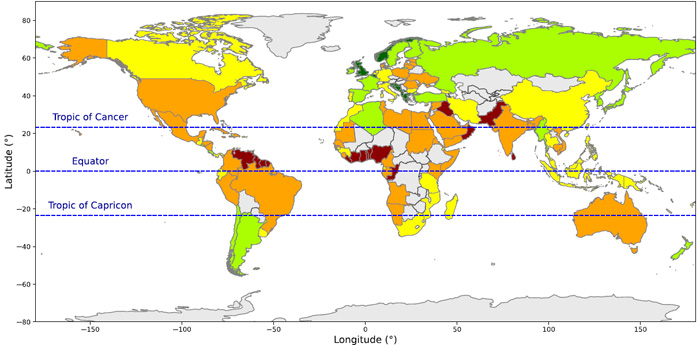
The figure above summarises the results of the CVI study on a country-by-country basis. Eurasia is surprisingly the least vulnerable continent in this respect, especially Britain and Norway that are so exposed to the fierce North Atlantic. That is partly due to those countries high adaptive capacity and communal resilience, but mainly to their rugged and deeply indented western coasts; a legacy of glaciation. It’s important to note that coloration on the figure can be misleading. For instance, the higher resolution data pinpoint extremely high vulnerability of stretches of coast dominated by low-lying deltas, such as those of Pakistan, India, Myanmar and SE Asia. Equally surprising is the high vulnerability of North America at similar latitudes; somewhat ironic for the heartland of climate-change denial. High resolution also points to counterintuitive hazards; for instance coastal defences sometimes exacerbate vulnerability by increasing erosion on nearby undefended stretches and by hindering sediment movement. Increased onshore infrastructure boosts runoff and erosion in the coastal realm and displaces natural buffers, such as coastal forest, to storm surges: perhaps partly responsible for the high vulnerability of coasts around the hurricane belt of the Gulf of Mexico and Caribbean. Of the nineteen countries with greatest vulnerability 12 are in West Africa and NE South America and 2 in the Caribbean area. The paper is well worth reading, to get a flavour of the complexity involved and the vast magnitude of the task of ameliorating risk of coastal devastation that lies ahead in the next decades.
See especially: Global Coastal Vulnerability: Key Causes Revealed. Scienmag, 14 January 2026.