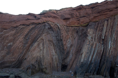
The northwest of Scotland has been a magnet to geologists for more than a century. It is easily accessed, has magnificent scenery and some of the world’s most complex geology. The oldest and structurally most tortuous rocks in Europe – the Lewisian Gneiss Complex – which span crustal depths from its top to bottom, dominate much of the coast. These are unconformably overlain by a sequence of mainly terrestrial sediments of Meso- to Neoproterozoic age – the Torridonian Supergroup – laid down by river systems at the edge of the former continent of Laurentia. They form a series of relic hills resting on a rugged landscape carved into the much older Lewisian. In turn they are capped by a sequence of Cambrian to Lower Ordovician shallow-marine sediments. A more continuous range of hills no more than 20 km eastward of the coast hosts the famous Moine Thrust Belt in which the entire stratigraphy of the region was mangled between 450 and 430 million years ago when the elongated microcontinent of Avalonia collided with and accreted to Laurentia. Exposures are the best in Britain and, because of the superb geology, probably every geologist who graduated in that country visited the area, along with many international geotourists. The more complex parts of this relatively small area have been mapped and repeatedly examined at scales larger than 1:10,000; its geology is probably the best described on Earth. Yet, it continues to throw up dramatic conclusions. However, the structurally and sedimentologically simple Torridonian was thought to have been done and dusted decades ago, with a few oddities that remained unresolved until recently.
Grossly simplified geological map of NW Scotland (credit: British Geological Survey)
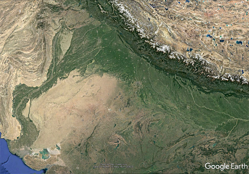
Active sedimentation in the Indus and Upper Ganges plains (green vegetated) derived from rapid erosion of the Himalaya (credit: Google Earth)
The Proterozoic Eon of the Precambrian is subdivided into the Palaeo-, Meso- and Neoproterozoic Eras that are, respectively, 900, 600 and 450 Ma long. The degree to which geoscientists are sufficiently interested in rocks within such time spans is roughly proportional to the number of publications whose title includes their name. Searching the ISI Web of Knowledge using this parameter yields 2000, 840 and 2700 hits in the last two complete decades, that is 2.2, 1.4 and 6.0 hits per million years, respectively. Clearly there is less interest in the early part of the Proterozoic. Perhaps that is due to there being smaller areas over which they are exposed, or maybe simply because what those rocks show is inherently less interesting than those of the Neoproterozoic. The Neoproterozoic is stuffed with fascinating topics: the appearance of large-bodied life forms; three Snowball Earth episodes; and a great deal of tectonic activity, including the Pan-African orogeny. The time that precedes it isn’t so gripping: it is widely known as the ‘boring billion’ – coined by the late Martin Brazier – from about 1.75 to 0.75 Ga. The Palaeoproterozoic draws attention by encompassing the ‘Great Oxygenation Event’ around 2.4 Ga, the massive deposition of banded iron formations up to 1.8 Ga, its own Snowball Earth, emergence of the eukaryotes and several orogenies. The Mesoproterozoic witnesses one orogeny, the formation of a supercontinent (Rodinia) and even has its own petroleum potential (93 billion barrels in place in Australia’s Beetaloo Basin. So it does have its high points, but not a lot. Although data are more scanty than for the Phanerozoic Eon, during the Mesoproterozoic the Earth’s magnetic field was much steadier than in later times. That suggests that motions in the core were in a ‘steady state’, and possibly in the mantle as well. The latter is borne out by the lower pace of tectonics in the Mesoproterozoic. Continue reading “The effect of surface processes on tectonics”→
We have become accustomed to thinking that up to 90% of organisms were snuffed out by the catastrophe at the Permian-Triassic boundary 252 Ma ago. Those are the figures for marine organisms, whose record in sediments is the most complete. It has also been estimated to have lasted a mere 60 ka, and the recovery in the Early Triassic to have taken as long as 10 Ma. There are hints of three separate pulses of extinction related to: initial gas emission from the Siberian Traps; coal fires; and release of methane from sea-floor gas hydrates at the peak of global warming. Various terrestrial sequences record the collapse of dense woodlands, so that the Early Triassic is devoid of coals that are widespread in the preceding Late Permian. A new detailed study of terrestrial sediments in the Sydney Basin of eastern Australia reveals something new (Fielding, C.R. and 10 others 2019. Age and pattern of the southern high-latitude continental end-Permian extinction constrained by multiproxy analysis. Nature Communications, v. 10, online publications: DOI: 10.1038/s41467-018-07934-z).
The distinctive, tongue-like form of Glossopteris leaves that dominate the coal-bearing Permian strata of the southern coninents. Their occurrence in South America, Africa, India, Australia, New Zealand, and Antarctica prompted Alfred Wegener to suggest that these modern continents had been united in Pangaea by Permian times: a key to continental drift. (Credit: Getty Images)
Christopher Fielding or the University of Nebraska-Lincoln and colleagues focused on pollens, geochemistry and detailed dating of the sedimentary succession across the P-Tr boundary exposed on the New South Wales coast. The stratigraphy is intricately documented by a 1 km deep well core that penetrates a more or less unbroken fluviatile and deltaic sequence that contains eleven beds of volcanic ash. The igneous layers are key to calibrating age throughout the sequence (259.10 ± 0.17 to 247.87 ± 0.11 Ma using zircon U-Pb methods). The pollens change abruptly from those of a Permian flora, dominated by tongue-like glossopterid plants, to a different association that includes conifers. The change coincides with a geochemical ‘spike’ in the abundance of nickel and a brief change in the degree of alteration of detrital fledspars to clay minerals. The first implicates the delivery of massive amounts of nickel to the atmosphere, probably by the eruption of the Siberian Traps , which contain major economic nickel deposits. The second feature suggests a brief period of warmer and more humid climatic conditions. A third geochemical change is the onset of oscillations in the abundance of 13C that are thought to record major changes in plant life across the planet. These features would have been an easily predicted association with the 252 Ma mass extinction were it not for the fact that the radiometric dating places them about 400 thousand years before the well-known changes in global animal life. Detailed dating of the Siberian Traps links the collapse of Glossopteris and coal formation to the earliest extrusion of flood basalts, which suggests that the animal extinctions were driven by cumulative effects of the later outpourings
Radiocarbon dating is the most popular tool for assessing the ages of archaeological remains and producing climatic time series, as in lake- and sea-floor cores, provided that organic material can be recovered. Its precision has steadily improved, especially with the development of accelerator mass spectrometry, although it is still limited to the last 50 thousand years or so because of the short half-life of 14C (about 5,730 years,). The problem with dating based on radioactive 14C is its accuracy; i.e. does it always give a true date. This stems from the way in which 14C is produced – by cosmic rays interacting with nitrogen in the atmosphere. Cosmic irradiation varies with time and, consequently, so does the proportion of 14C in the atmosphere. It is the isotope’s proportion in atmospheric CO2 gas at any one time in the past, which is converted by photosynthesis to dateable organic materials, that determines the proportion remaining in a sample after decay through the time since the organism died and became fossilised. Various approaches have been used to allow for variations in 14C production, such as calibration to the time preserved in ancient timber by tree rings which can be independently radiocarbon dated. But that depends on timber from many different species of tree from different climatic zones, and that is affected by fractionation between the various isotopes of carbon in CO2, which varies between species of plant. But there is a better means of calibration.
The carbonate speleothem that forms stalactites and stalagmites by steady precipitation from rainwater, sometimes to produce visible layering, not only locks in 14C dissolved from the atmosphere by rainwater but also environmental radioactive isotopes of uranium and thorium. So, layers in speleothem may be dated by both methods for the period of time over which a stalagmite, for instance, has grown. This seems an ideal means of calibration, although there are snags; one being that the proportion of carbon in carbonates is dominated by that from ancient limestone that has been dissolved by slightly acid rainwater, which dilutes the amount of 14C in samples with so called ‘dead carbon’. Stalagmites in the Hulu Cave near Nanjing in China have particularly low dead-carbon fractions and have been used for the best calibrations so far, going back the current limit for radiocarbon dating of 54 ka (Cheng, H. and 14 others 2018. Atmospheric 14C/12C during the last glacial period from Hulku Cave. Science, v. 362, p. 1293-1297; DOI: 10.1126/science.aau0747). Precision steadily falls off with age because of the progressive reduction to very low amounts of 14C in the samples. Nevertheless, this study resolves fine detail not only of cosmic ray variation, but also of pulses of carbon dioxide release from the oceans which would also affect the availability of 14C for incorporation in organic materials because deep ocean water contains ‘old’ CO2.
My first field trip from the Geology Department at the University of Birmingham in autumn 1964 was located within hooter distance of the giant British Leyland car plant at Longbridge. It involved a rubbish-filled linear quarry behind a row of shops on the main road through south Birmingham. Not very prepossessing but it clearly exposed a white quartzite, which we were told was a beach deposit laid down by a massive marine transgression at the start of the Cambrian. An hour later we were shown an equally grim exposure of weathered volcanic rocks in the Lickey Hills; they were a sort of purple brown, and said to be Precambrian in age. Not an excellent beginning to a career, but from time to time other Cambrian quartzites sitting unconformably on Precambrian rocks entered our field curriculum: in the West Midlands, Welsh Borders and much further afield in NW Scotland, as it transpired on what had been two separate continental masses of Avalonia and Laurentia. This had possibly been a global marine transgression.
In North America, then the Laurentian continent, what John Wesley Powell dubbed the Great Unconformity in the Grand Canyon has as its counterpart to the Lickey Quartzite the thrillingly named Tonto Group of the Lower Cambrian resting on the Vishnu Schists that are more than a billion years older. Part of the Sauk Sequence, the Tonto Group is, sadly, not accompanied by the Lone Ranger Group, but the Cambrian marine transgression crops out across the continent. In fact it was a phenomenon common to all the modern continents. Global sea level rose relative to the freeboard of the continents then existing. A recent study has established the timing for the Great Unconformity in the Grand Canyon by dating detrital zircons above and below the unconformity (Karlstrom, K, et al. 2018. Cambrian Sauk transgression in the Grand Canyon region redefined by detrital zircons. Nature Geoscience, v. 11, p. 438-443; doi:10.1038/s41561-018-0131-7). Rather than starting at the outset of the Cambria at 542 Ma, the marine transgression was a protracted affair that began around 527 Ma with flooding reaching a maximum at the end of the Cambrian.
Extensive flooding of the continents at the end of the Cambrian (credit: Ron Blakey , Colorado Plateau Geosystems)
It seems most likely that the associated global rise in sea level relative to the continents was a response to the break-up of the Rodinia supercontinent by considerable sea-floor spreading. The young ocean floor, having yet to cool to an equilibrium temperature, would have had reduced density so that the average depth of the ocean basins decreased, thereby flooding the continents. The creation of vast shallow seas across the continents has been suggested to have been a major factor in the explosive evolution of Cambrian shelly faunas, partly by expanding the range of ecological niches and partly due to increased release of calcium ions to to seawater as a result of chemical weathering.
A fully revised edition of Steve Drury’s book Stepping Stones: The Making of Our Home World can now be downloaded as a free eBook
The longest and most extreme glacial epoch during the Phanerozoic took place between 360 and 260 Ma ago, when it dominated the Carboniferous and Permian sedimentary sequences across the planet. On continents that lay athwart the Equator during these times, sedimentation was characterised by cycles between shallow marine and terrestrial conditions. These are epitomised by the recurring ‘Coal-Measure’ cyclothem of, from bottom to top: open-sea limestone; near-shore marine mudstone; riverine sandstone; coal formed in swamps. This sequence represents a rapid rise in sea level as ice sheets melted, sustained during an interglacial episode and then falling sea level as ice once again accumulated on land to culminate in a glacial maximum when coal formed in coastal mires. During the Late Palaeozoic Era a single supercontinent extended from pole to pole. The break-up of Pangaea was charted by Alfred Wegener in 1912, partly by his using glacial deposits and ice-gouged striations on the southern continents. With the present widely separated configuration of major landmasses glacial sediments and the directions of inferred ice movements could only be reconciled by reassembling Africa, India, South America, Antarctica and Australia in the form of a single, congruent southern continent that he called Gondwanaland. In Wegener’s reconstruction the glacial features massed together on Gondwanaland with the striations radiating outwards from what would then have been the centre of a huge ice cap.
There are many localities on the present southern continents where such striations can be seen on the surface of peneplains etched into older rocks that underlie Carboniferous to Permian tillites, but later erosion has removed the continuity of the original glacial landscape. There are, however, some parts of central Africa where it is preserved. By using the high-resolution satellite images (with pixels as small as 1 m square) that are mosaiced together in Google Earth, Daniel Paul Le Heron of Royal Holloway, University of London has revealed a series of 1 to 12 km wide sinuous belts in a 6000 km2 area of eastern Chad that are superimposed unconformably on pre-Carboniferous strata (Le Heron, D.P. 2018. An exhumed Paleozoic glacial landscape in Chad. Geology, v.46(1), p. 91-94; doi:10.1130/G39510.1). They comprise irregular tracts of sandstone to the south of a major Carboniferous sedimentary basin. Zooming in to them (try using 17.5° N 22.25°E as a search term in Google Earth) reveals surfaces dominated by wavy, roughly parallel lines. Le Heron interprets these as mega-scale glacial lineations, formed by ice flow across underlying soft Carboniferous glacial sediments as seen in modern glacial till landforms in Canada. In places they rest unconformably on older rocks, sometimes standing above the level of the sandstone plateaux as relics of what may have been nunataks. There are even signs of elliptical drumlins.
An oblique Google Earth view looking to the south-east shows mega-scale glacial lineations from a glacial flow way in eastern Chad. The lower-right quadrant shows the unconformity atop older bedded strata that are dipping to the west. Click on the image to see a full resolution view. (Credit: Google Earth)
Glacial tillites and glaciofluvial sediments of Late Palaeozoic age are common across the Sahara and in the Sahelian belt, but in areas as remote as those in eastern Chad. So a systematic survey using the resolving power of Google Earth may well yield yet more examples. It is tedious work in such vast areas, unless, of course, one bears in mind Alfred Wegener, the founder of the hypothesis of continental drift and ‘Big’ Earth Science as a whole, who would have been gleeful at the opportunity.
A fully revised edition of Steve Drury’s book Stepping Stones: The Making of Our Home World can now be downloaded as a free eBook
During most of the last hundred years every car body, rebar rod in concrete, ship, bridge and skyscraper frame had its origins in vividly striped red rocks from vast open-pit mines. Comprising mainly iron oxides with some silica, these banded iron formations, or BIFs for short, occur in profitable tonnages on every continent.
2.1 billion years old boulder of banded ironstone. (credit: Wikipedia)
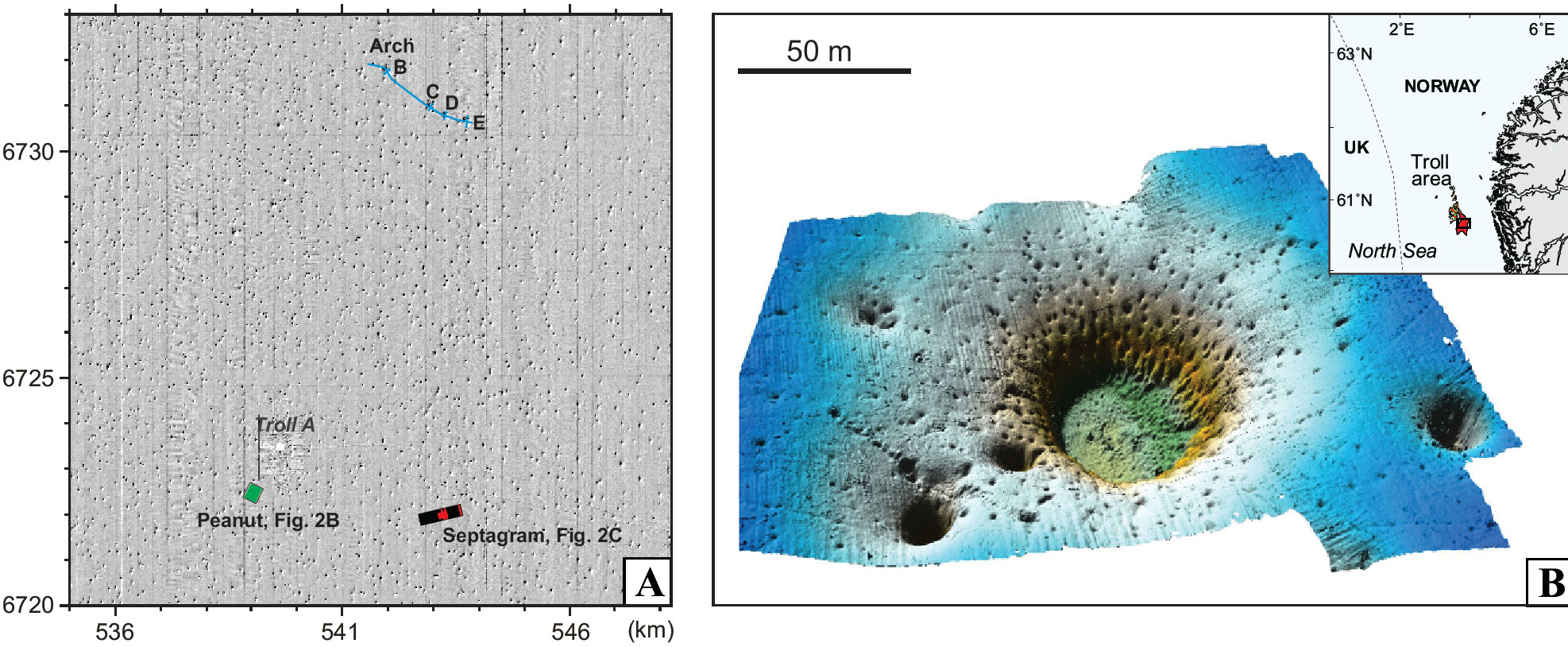
Detailed acoustic imaging above the Troll gas field in the northern North Sea off western Norway has revealed tens of thousands of elliptical pits on the seabed. At around 10 to 20 per square kilometre over an area of about 15,000 km2 there are probably between 150 to 300 thousand of them. They range between 10 to 100 m across and are about 6 m deep on average, although some are as deep as 20 m. They are pretty much randomly distributed but show alignment roughly parallel to regional N-S sea-floor currents. Many of the world’s continental shelves display such pockmark fields, but the Troll example is among the most extensive. Almost certainly the pockmarks formed by seepage of gas or water to the surface. However, detailed observations suggest they are inactive structures with no sign of bubbles or fluid seepage. Yet the pits cut though glacial diamictites deposited by the most recent Norwegian Channel Ice Stream through which icebergs once ploughed and which is overlain by thin Holocene marine sediments. One possibility is that they record gas loss from the Troll field, another being destabilisation of shallow gas hydrate deposits.
Parts of the Troll pockmark field off Norway. A: density of pockmarks in an area of 169 square km. B: details of a cluster of pockmarks. (Credit: Adriano Mazzini, Centre for Earth Evolution and Dynamics (CEED) University of Oslo)
Norwegian geoscientists have studied part of the field in considerable detail, analysing carbonate-rich blocks and foraminifera in the pits (Mazzini, A. and 8 others 2017. A climatic trigger for the giant Troll pockmark field in the northern North Sea. Earth and Planetary Science Letters, v. 464, p. 24-34; http://dx.doi.org/10.1016/j.epsl.2017.02.014). The carbonates show very negative δ13C values that suggest the carbon in them came from methane, which could indicate either of the two possible means of formation. However, U-Th dating of the carbonates and radiocarbon ages of forams in the marine sediment infill suggest that they formed at around 10 ka ago; 1500 years after the end of the Younger Dryas cold episode and the beginning of the Holocene interglacial. Most likely they represent destabilisation of a once-extensive, shallow layer of methane hydrates in the underlying sediments, conditions during the Younger Dryas having been well within the stability field of gas hydrates. Sporadic leaks from the deeper Troll gas field hosted by Jurassic sandstones is unlikely to have created such a uniform distribution of gas-release pockmarks. Adriano Mazzini and colleagues conclude that rapid early Holocene warming led to sea-floor temperatures and pressures outside the stability field of gas hydrates. There are few signs that hydrates linger in the area, explaining the present inactivity of the pockmarks – all the methane and CO2 escaped before 10 ka.
Gas hydrates are thought to be present beneath shallow seas today, wherever sea-floor sediments have a significant organic carbon content and within the pressure-temperature window of stability of these strange ice-like materials. Mazzini et al.’s analysis of the Troll pockmark field clearly has profound implications for the possible behaviour of gas hydrates at a time of global climatic warming. As well as their destabilisation adding to methane release from onshore peat deposits currently locked by permafrost and a surge in global warming, there is an even more catastrophic possibility. The whole of the seaboard of the southern North Sea was swept by a huge tsunami about 8000 years ago, which possibly wiped out Mesolithic human occupancy of lowland Britain, the former land mass of Doggerland, and the ‘Low Countries’ of western Europe. This was created by a massive submarine landslide – the Storegga Slide just to the north of the Troll field – which may have been triggered by destabilisation of submarine gas hydrates during early Holocene warming of the oceans.
It is widely known that glacial ice contains a record of Earth’s changing atmospheric composition in the form of bubbles trapped when the ice formed. That is fine for investigations going back about a million years, in particular those that deal with past climate change. Obviously going back to the composition of air tens or hundreds of million years ago cannot use such a handy, direct source of data, but has relied on a range of indirect proxies. These include the number of pores or stomata on fossil plant leaves for CO2, variations in sulfur isotopes for oxygen content and so on. Variation over time of the atmosphere’s content of oxygen has vexed geoscientists a great deal, partly because it has probably been tied to biological evolution: forming by some kind of oxygenic photosynthesis and being essential for the rise to dominance of eukaryotic animals such as ourselves. Its presence or absence also has had a large bearing on weathering and the associated dissolution or precipitation of a variety of elements, predominantly iron. Despite progressively more clever proxies to indicate the presence of oxygen, and intricate geochemical theory through which its former concentration can be modelled, the lack of an opportunity to calibrate any of the models has been a source of deep frustration and acrimony among researchers.
Yet as is often said, there are more ways of getting rid of cats than drowning them in butter. The search has been on for materials that trap air in much the same way as does ice, and one popular, if elusive target has been the bubbles in crystals of evaporite minerals. The trouble is that most halite deposits formed by precipitation of NaCl from highly concentrated brines in evaporating lakes or restricted marine inlets. As a result the bubbles contain liquids that do a grand job of preserving aqueous geochemistry but leave a lot of doubt as regards the provenance of gases trapped within them. For that to be a sample of air rather than gases once dissolved in trapped liquid, the salt needs to have crystallized above the water surface. That may be possible if salt forms from brines so dense that crystals are able to float, or perhaps where minerals such as gypsum form as soil moisture is drawn upwards by capillary action to form ‘desert roses’. A multinational team, led by Nigel Blamey of Brock University in Canada, has published results from Neoproterozoic halite whose chevron-like crystals suggest subaerial formation (Blamey, N.J.F. and 7 others, 2016. Paradigm shift in determining Neoproterozoic atmospheric oxygen. Geology, v. 44, p. 651-654). Multiple analyses of five halite samples from an ~815 Ma-old horizon in a drill core from the Neoproterozoic Canning Basin of Western Australia contained about 11% by volume of oxygen, compared with 25% from Cretaceous salt from China, 20% of late-Miocene age from Italy, and 19 to 22% from samples modern salt of the same type.
Evaporite salts in the Salar de Atacama Chile (credit: Wikipedia)
Although the Neoproterozoic result is only about half that present in modern air, it contradicts results that stem from proxy approaches, which suggest a significant rise in atmospheric oxygenation from 2 to about 18% during the younger Cryogenian and Ediacaran Periods of the Neoproterozoic, when marine animal life made explosive developments at the time of repeated Snowball Earth events. Whether or not this approach can be extended back to the Great Oxygenation Event at around 2.3 Ga ago and before depends on finding evaporite minerals that fit stringent criteria for having formed at the surface: older deposits are known even from the Archaean.
Readers may recall my occasional rants over the years against the growing bandwagoning for an ‘Anthropocene‘ epoch at the top of the stratigraphic column. I , for one, was delighted to find in the latest issue of GSA Today a more sober assessment of the campaign by two stratigraphers who are well placed to have a real say in whether or not the ‘Anthropocene’ is acceptable, one serving on the International Commission on Stratigraphy, the other on the North American Commission on Stratigraphic Nomenclature (Finney, S.C. & Edwards, L.E. 2016. The “Anthropocene” epoch: Scientific decision or political statement? GSA Today, v. 26 (3–4).
At the end of the 1970’s I was invited by the Deputy Director of the Geological Survey of India (Southern Region) to participate in the Great Postal Symposium on the Cuddapah Basin: a sort of harbinger of the Internet and Skype, but using snail-mail. Feeling pretty honoured and most intrigued I accepted; not that I knew the first thing about the subject. A regular stream of foolscap mimeographed contributions kept me nipping out of my office to check my pigeon hole for about 6 months. I learned a lot, but felt unable to comment. Four years on I was taken across the Cuddapahs by my first research student – a budding moto-cross driver with a morbid fear of bullock carts – en route from the Archaean low-grade greenstone-granite terrains of Karnataka for a peek at the fabled charnockites near Chennai (then Madras). A bit of a round-about route but spurred by my memories of the Great Postal Symposium. Sadly, the detour was marred for me by a severe case of sciatica brought on by manic driving, the state of the trans-Cuddapah highway and a misplaced gamma-globulin shot to ward off several varieties of hepatitis: I mainly blamed the nurse who demanded that I drop my drawers and bravely take the huge needle in a buttock – they do these things more humanely these days. Anyhow, apart from seeing many dusty villages build of slates perfect enough to make a full-size snooker table, my mind was elsewhere and I have long regretted that.
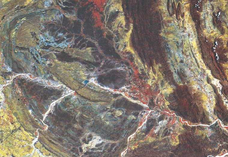
Landsat image mosaic showing part of the Cuddapah Basin.
Hosting possibly the world’s only diamondiferous Precambrian conglomerate, the Cuddapah Basin contains a 5 km thickness of diverse sedimentary strata, but no tangible fossils. It rests unconformably on the Archaean greenstone-granite terrain of the Dharwar Craton and so is Proterozoic in age; an Eon that spans 2 billion years. The middle of the lowest sedimentary formations (the Papaghni and Chitravati Groups) contains volcanic rocks dated at ~1.9 Ga; another group is cut by a ~1.5 Ga granite, and hitherto the youngest dateable event is the emplacement of 1.1 Ga kimberlites that sourced the diamonds in the conglomerate. Until recently the stratigraphy has been known in some detail, but how to partition it in Proterozoic time is barely conceivable with just three dates in the middle parts that span 800 Ma. All that can be said about the base of the Cuddapah sediments is that they are younger than the 3.1 to 2.6 Ga Archaean rocks beneath. Since the uppermost beds are truncated by a huge thrust system that shoved deep crustal granulites over them their minimum age is equally vague.
Structurally, the Basin began to form on a stable continent underpinned by the Dharwar Craton, but when that collided with Enderbyland in Antarctica, as part of the accretion of the Gondwana supercontinent, sedimentation may have been in an entirely different setting. Indeed, some of the sediments have been carried over the undisturbed part of the basin by a major thrust system. To explore both sedimentary and tectonic evolution Australian, Indian and Canadian geoscientists combined to sample and radiometrically date the entire pile (Collins, A.S. and 13 others 2015. Detrital mineral age, radiogenic isotopic stratigraphy and tectonic significance of the Cuddapah Basin, India. Gondwana Research, v. 28, p. 1294-1309). By precisely dating detrital micas and zircons from the sediments the team was able to check the source region of sedimentary grains as well as to establish a maximum age for each major stratigraphic unit. This helped establish a 3-part sedimentary and tectonic history. The earliest sediments came from the cratonic area to the west, but there are signs that collisional orogeny between 1590 and 1659 Ma produced a new sedimentary source in metamorphic rocks forming to the east. A return to westward provenance marked the youngest sedimentary setting. This enabled the team to suggest a dual evolution of the Basin, first as an extensional rift opening at the east of what is now the Dharwar craton followed by collisional orogeny that transformed the setting to that of a foreland basin, analogous to the Molasse basin in front of the Alps during Cenozoic times, ending with tectonic inversion when extension changed to compression and thrusting.
But to what extent did the work improve the age subdivision of the Cuddapah Basin? Apparently very little, which may be down to a problem with dating detrital minerals. If magmatic and metamorphic evolution was continuous in the areas from which sediments moved, then the youngest grain is a good guide to the maximum age of the sediment being analysed. The more strata are analysed in this way the better the detail of sedimentary timing. But two tectonic terrains are unlikely to produce zircons time and time again during a period approaching a billion years. The data indicate only 3 or 4 episodes of ‘zirconogenesis’ in the sedimentary hinterlands, between about 900 to 1940 Ma. Apart from helping correlate sedimentary formations that were previously deemed stratigraphically different – which did help in tectonically unravelling this complex major feature – several hundred isotopic analyses of zircons and micas have give much the same timing as was known already in more precise terms from stratigraphy assisted by a few dozen conventional radiometric dates.
Many of the vast wastes of northern Canada and Scandinavia that were ground to a paste by ice sheets during the last glacial cycle show peculiar features that buck the general glacial striation of the Shield rocks. They are round-topped ridges that wind apparently aimlessly across the tundra. In what is now a gigantic morass, the ridges form well-drained migration routes for caribou and became favourite hunting spots for the native hunter gatherers: in Canada they are dotted with crude simulations of the human form, or inugoks, that the Innuit erected to corral game to killing grounds. Where eroded they prove to be made of sand and gravel, which has proved an economic resource in some areas lacking in building aggregate, good but small examples being found in the Scottish Midland Valley that have served development of Glasgow and Edinburgh. They were given the Gaelic name eiscir meaning ‘ridge of gravel’ (now esker) from a few examples in Ireland.
Eskers form from glacial meltwater that makes its way from surface chasms known as moulins to the very bottom of an ice sheet where water flows much in the manner of a river, except in tubes rather than channels. Where the ice base is more or less flat the tubes meander as do normal sluggish rivers, and like them the tubes deposit a proportion of the abundant sediment derived by melting glacial ice. Once the ice sheet melts and ablates away, the sediments lose the support of the tube walls and flop down to form the eponymous low ridges: the reverse of the sediment filled channels of streams that have either dried up or migrated. Eskers are one of the features that shout ‘glacial action’ with little room for prevarication.
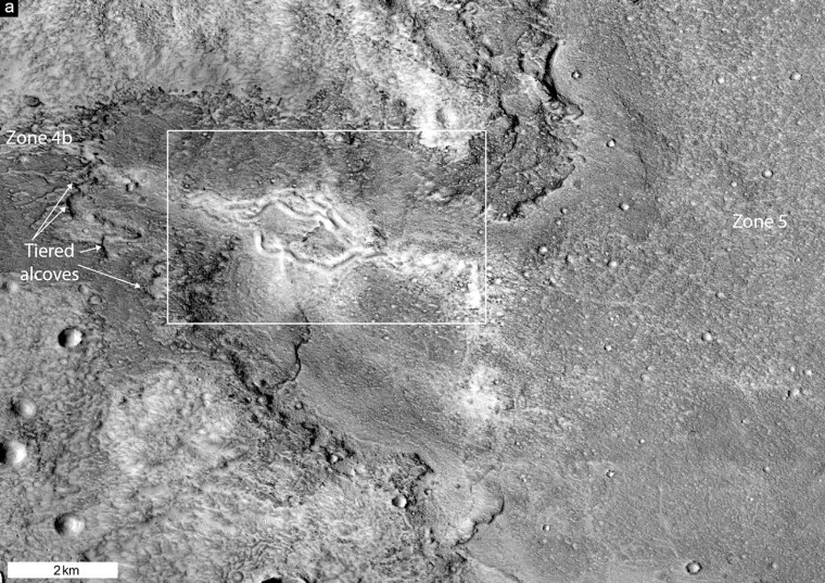
The classic form of eskers in the Phlegra Montes of Mars. (credit: Figure 6 in Gallagher and Balme, 2015)
Glacial terrains on Mars have been proposed for some odd looking surfaces, but other processes such as debris flows are equally attractive. To the astonishment of many, Martian eskers have now been spotted during systematic interpretation of the monumental archives of high-resolution orbital images of the planetary surface (Gallagher, C. & Balme, M. 2015. Eskers in a complete, wet-based glacial system in the Phlegra Montes region, Mars. Earth and Planetary Science Letters, v. 431, p. 96-109). The discovery is in a suspected glacial terrain that exhibits signs of something viscous having flowed on low ground around higher topographic features, bombardment stratigraphy suggests a remarkable young age for the terrain or about 150 Ma ago: the Amazonian. Ice and its effects are not too strange to suggest for Mars which today is pretty much frigid, except for a few suggestions of active flow of small watery streams. Eskers demand meltwater in abundance, and Gallagher and Balme attribute some of the other features in the Phlegra Montes to wet conditions. However, the eskers are a one-off, so far as they know. Consequently, rather than appealing to some climatic warm up to explain the evidence for wetness, they suggest that the flowing water tubes resulted from melting deep in the ice as a result of locally high heat flow through the Martian crust, which is a lot more plausible.
The main source for iron and steel has for more than half a century been Precambrian rock characterised by intricate interlayering of silica- and iron oxide-rich sediments known as banded iron formations or BIFs. They always appear in what were shallow-water parts of Precambrian sedimentary basins. Although much the same kind of material turns up in sequences from 3.8 to 0.6 Ga, by far the largest accumulations date from 2.6 to 1.8 Ga, epitomised by the vast BIFs of the Palaeoproterozoic Hamersley Basin in Western Australia. This peak of iron-ore deposition brackets the time (~2.4 Ga) when world-wide evidence suggests that the Earth’s atmosphere first acquired tangible amounts of free oxygen: the so-called ‘Great Oxidation Event’. Yet the preservation of such enormous amounts of oxidised iron compounds in BIFs is paradoxical for two reasons: the amount of freely available atmospheric oxygen at their acme was far lower than today; had the oceans contained much oxygen, dissolved ions of reduced Fe-2 would not have been able to pervade seawater as they had to for BIFs to have accumulated in shallow water. Iron-rich ocean water demands that its chemical state was highly reducing.
Oblique view of an open pit mine in banded iron formation at Mount Tom Price, Hamersley region Western Australia (Credit Google earth)
The paradox of highly oxidised sediments being deposited when oceans were highly reduced was resolved, or seemed to have been, in the late 20th century. It involved a hypothesis that reduced, Fe-rich water entered shallow, restricted basins where photosynthetic organisms – probably cyanobacteria – produced localised enrichments in dissolved oxygen so that the iron precipitated to form BIFs. Later work revealed oddities that seemed to suggest some direct role for the organisms themselves, a contradictory role for the co-dominant silica-rich cherty layers and even that another kind of bacteria that does not produce oxygen directly may have deposited oxidised iron minerals. Much of the research focussed on the Hamersley BIF deposits, and it comes as no surprise that another twist in the BIF saga has recently emerged from the same, enormous repository of evidence (Rasmussen, B. et al. 2015. Precipitation of iron silicate nanoparticles in early Precambrian oceans marks Earth’s first iron age. Geology, v. 43, p. 303-306).
The cherty laminations have received a great deal less attention than the iron oxides. It turns out that they are heaving with minute particles of iron silicate. These are mainly the minerals stilpnomelane [K(Fe,Mg)8(Si, Al)12(O, OH)27] and greenalite [(Fe)2–3Si2O5(OH)4] that account for up to 10% of the chert. They suggest that ferruginous, silica-enriched seawater continually precipitated a mixture of iron silicate and silica, with cyclical increases in the amount of iron-silicate. Being such a tiny size the nanoparticles would have had a very high surface area relative to their mass and would therefore have been highly reactive. The authors suggest that the present mineralogy of BIFs, which includes iron carbonates and, in some cases, sulfides as well as oxides may have resulted from post-depositional mineral reactions. Much the same features occur in 3.46 Ga Archaean BIFs at Marble Bar in Western Australia that are almost a billion years older that the Hamersley deposits, suggesting that a direct biological role in BIF formation may not have been necessary.
The made-up word chrononymy could be applied to the study of the names of geological divisions and their places on the International Stratigraphic Chart. Until 2008 that was something of a slow-burner, as careers go. It all began with Giovanni Arduino and Johann Gotlob Lehman in the mid- to late 18th century, during the informal historic episode known as the Enlightenment. To them we owe the first statements of stratigraphic principles and the beginning of stratigraphic divisions: rocks divided into the major segments of Primitive, Secondary, Tertiary and Quaternary (Arduino). Thus stratigraphy seeks to set up a fundamental scale or chart for expressing Earth’s history as revealed by rocks. The first two divisions bit the dust long ago; Tertiary is now an informal synonym for the Cenozoic Era; only Quaternary clings on as the embattled Period at the end of the Cenozoic. All 11 Systems/Periods of the Phanerozoic, their 37 Series/Epochs and 85 Stages/Ages in the latest version of the International Stratigraphic Chart have been thrashed out since then, much being accomplished in the late 19th and early 20th centuries. Curiously, the world body responsible for sharpening up the definition of this system of ‘chrononymy’, the International Commission on Stratigraphy (ICS), seems not to have seen fit to record the history of stratigraphy: a great mystery. Without it geologists would be unable to converse with one another and the world at large.
Yet now an increasing number of scientists are seriously proposing a new entry at the 4th level of division after Eon, Era and Period: a new Epoch that acknowledges the huge global impact of human activity on atmosphere, hydrosphere, biosphere and even lithosphere. They want it to be called the Anthropocene, and for some its eventual acceptance ought to relegate the current Holocene Epoch, in which humans invented agriculture, a form of economic intercourse and exchange known as capital and all the trappings of modern industry, to the 5th division or Stage. Earth-pages has been muttering about the Anthropocene for the past decade, as charted in a number of the links above, so if you want to know which way its author is leaning and how he came to find the proposal an unnecessary irritation, have a look at them. Last week things became sufficiently serious for another comment. Simon Lewis and Mark Maslin of the Department of Geography at University College London have summarised the scientific grounds alleged to justify an Anthropocene Epoch and its strict definition in a Nature Perspective (Lewis, S.J. & Maslin, M.A. 2015. Defining the Anthropocene. Nature, v. 519, p. 171-180).-=, which is interestingly discussed in the same Issue by Richard Monastersky.
Lewis and Maslin present two dates that their arguments and accepted stratigraphic protocols suggest as candidates for the start of the Anthropocene: 1610 and 1964 CE, both of which relate to features that are expressed by geological records that should last indefinitely. The first is a decline and eventual recovery in the atmospheric CO2 level recorded in high-resolution Antarctic ice core records between 1570 and 1620 CE that can be ascribed to the decline in the population of the Americas’ native peoples from an estimated 60 to 6 million. This result of the impact of European first colonisation – disease, slaughter, enslavement and famine – reduced agriculture and fire use and saw the regeneration of 5 x 10⁷ hectares of forest, which drew down CO2 globally. It also coincides with the coolest part of the Little Ice Age from 1594-1677 CE. They caution against the start of the Industrial Revolution as an alternative for a ‘Golden Spike’ since it was a diachronous event, beginning in Europe. Instead, they show that the second proposal for a start in 1964 has a good basis in the record of global anthropogenic effects on the Earth marked by the peak fallout of radioactive isotopes generated by atomic weapons tests during the Cold War, principally 14C with a 5730 year half life, together with others more long-lived. The year 1964 is also roughly when growth in all aspects of human activity really took off, which some dub in a slightly Tolkienesque manner the ‘Great Acceleration’. [There is a growing taste for this kind of hyperbole, e.g. the ‘Great Oxygenation Event’ around 2.4 Ga and the ‘Great Dying’ for the end-Permian mass extinction]. Yet they neglect to note that the geochronological origin point for times past has been defined as 1950 CE when nucleogenic 14C contaminated later materials as regards radiocarbon dating, which had just become feasible. Lewis and Maslin conclude their Perspective as follows:
To a large extent the future of the only place where life is known to exist is being determined by the actions of humans. Yet, the power that humans wield is unlike any other force of nature, because it is reflexive and therefore can be used, withdrawn or modified. More widespread recognition that human actions are driving far-reaching changes to the life-supporting infrastructure of Earth may well have increasing philosophical, social, economic and political implications over the coming decades.
So the Anthropocene adds the future to the stratigraphic column, which seems more than slightly odd. As Richard Monastersky notes, it is in fact a political entity: part of some kind of agenda or manifesto; a sort of environmental agitprop from the ‘geos’. As if there were not dozens of rational reasons to change human impacts to haul society back from catastrophe, which many people outside the scientific community have good reason to see as hot air on which there is never any concrete action by ‘the great and the good’. Monastersky also notes that the present Anthropocene record in naturally deposited geological materials accounts for less than a millimetre at the top of ocean-floor sediments. How long might the proposed Epoch last? If action to halt anthropogenic environmental change does eventually work, the Anthropocene will be very short in historic terms let alone those which form the currency of geology. If it doesn’t, there will be nobody around able to document, let alone understand, the epochal events recorded in rocks. At its worst, for some alien, visiting planetary scientists, far in the future, an Anthropocene Epoch will almost certainly be far shorter than the 104 to 105 years represented by the hugely more important Palaeozoic-Mesozoic and Mesozoic-Cenozoic boundary sequences; but with no Wikipedia entry.
Not everybody gets a vote on these kinds of thing, such is the way that science is administered, but all is not lost. The final arbiter is the Executive Committee of the International Union of Geological Sciences (IUGS), but first the Anthropocene’s status as a new Epoch has to be approved by 60% of the ICS Subcommission on Quaternary Stratigraphy, if put to a vote. Then such a ‘supermajority’ would be needed from the chairs of all 16 of the ICS subcommissions that study Earth’s major time divisions. But first, the 37 members of the Subcommission on Quaternary Stratigraphy’s ‘Anthropocene’ working group have to decide whether or not to submit a proposal: things may drag on at an appropriately stratigraphic pace. Yet the real point is that the effect of human activity on Earth-system processes has been documented and discussed at length. I’ll give Marx the last word in this ‘The philosophers have only interpreted the world, in various ways. The point, however, is to change it’. A new stratigraphic Epoch doesn’t really seem to measure up to that…
Angular unconformity at Telheiro Beach, Portugal (credit: Gabriela Bruno)
This image posted at Earth Science Picture of the Day would be hard to beat as the definitive angular unconformity. It shows Upper Carboniferous marine metagreywackes folded during the Variscan orogeny overlain by Triassic redbeds. Structurally it is uncannily similar to Hutton‘s famous unconformity at Siccar Point on the coast of SE Scotland, although the tight folding there is Caledonian in age and the unconformable redbeds are Devonian in age.
One of the central measures used to describe modern ecosystems is the ratio of foliage area to that of the ground surface – the leaf area index (LAI) – which expresses the openness of vegetation canopies. A high LAI helps to retain moisture in the soil, partly by shading and cooling the surface to reduce evaporation and partly by stopping surface soil from being battered to a concrete-like consistency by heavy rain, which reduces the amount of water that can infiltrate. It is possible to estimate LAI across today’s entire land area using satellite image data but a proxy for palaeoecological LAI has remained hard to find.
Hemispherical photograph used to calculate modern canopy cover. (credit: Wikipedia; photo by S.B. Weiss)
The outer coating of leaves in well-shaded (high LAI) areas tends to have protective or pavement cells that are larger and have more complicated shapes than does that of leaves in more open canopies. The framework of leaf cells is silica-based and made up of structures known as phytoliths whose morphologies vary in much the same way as the cells that they support. So theoretically it is possible to use fossil phytoliths in terrestrial sediments to estimate LAI variations through time in local canopies, but first the approach needs a means of calibration from living ecosystems. The vegetation of Central American Costa Rica varies through the entire range of possible LAI values, which leads to varying amounts of sunlight available to the leaves of cover plants. Measuring the area and the degree of shape-complexity of phytoliths in modern soils there shows that each is positively correlated with LAI.
A modern herbivorous mammal (lowland paca) from dense forest in Costa Rica. (Photo credit: Wikipedia)
Putting this approach to use in the Cenozoic terrestrial sediments of Patagonia, US and Argentinean palaeoecologists aimed to examine how the evolution of the teeth of herbivorous mammals – a major feature in their speciation – linked to changes in vegetation structure (Dunn, R.E. et al. 2015. Linked canopy, climate and faunal change in the Cenozoic of Patagonia. Science, v. 347, p. 258-261). Using phytoliths they were able to show that in the Eocene the area was covered by dense, closed forest canopies that gradually became more open towards the end of the Eocene to be replaced by open forest and shrubland habitats in the Oligocene and Miocene, with a brief period of regreening. It was during the period of more open vegetation that tooth structure underwent the most change. Chances are that the vegetation shifts began in response to the onset of Antarctic glaciation at the beginning of the Oligocene Epoch and related climate change at the northern margin of the Southern Ocean. Changes in the herbivore teeth may have been in response to the increasing amount of dust adhering to leaves as canopies became more open and soil increasingly dried out.
Relative age sequences in sequences of fossiliferous sediments are frequently intricate, thanks to animal groups that evolved quickly to leave easily identifiable fossil species. Yet converting that one-after-the-other dating to absolute values of past time has been difficult and generally debateable. Up to now it has relied on fossil-based correlation with localities where parts of the sequence of interest interleave with volcanic ashes or lavas that can be dated radiometrically. Igneous rocks can provide reference points in time, so that age estimates of intervening sedimentary layers emerge by assuming constant rates of sedimentation and of faunal speciation. However, neither rate can safely be assumed constant, and those of evolutionary processes are of great biological interest.
Sunset at St Hilda’s Abbey, Whitby NE England; fabled haunt of Count Dracula (credit: epicnom)
If only we could date the fossils a wealth of information would be accessible. In the case of organisms that apparently evolved quickly, such as the ammonites of the Mesozoic, time resolution might be extremely fine. Isotopic analysis methods have become sufficiently precise to exploit the radioactive decay of uranium isotopes, for instance, at the very low concentrations found in sedimentary minerals such as calcium carbonate. So this prospect of direct calibration might seem imminent. Geochemists and palaeontologists at Royal Holloway University of London, Leicester University and the British Geological Survey have used the U-Pb method to date Jurassic ammonites (Li, Q. et al. 2014. U–Pb dating of cements in Mesozoic ammonites. Chemical Geology, v. 376, p. 76-83). The species they chose are members of the genus Hildoceras, familiar to junior collectors on the foreshore below the ruined Abbey of St Hilda at the small port of Whitby, in NE England. The abundance and coiled shape of Hildoceras was once cited as evidence for the eponymous founder of the Abbey ridding this choice locality of a plague of venomous serpents using the simple expedient of divine lithification.
Hildoceras from the Toarcian shales of Whitby (credit: Wikipedia)
The target uranium-containing mineral is the calcite formed on the walls of the ammonites’ flotation chambers either while they were alive or shortly after death. This early cement is found in all well-preserved ammonites. The Hildoceras genus is found in one of the many faunal Zones of the Toarcian Age of the Lower Jurassic; the bifrons Zone (after Hildoceras bifrons). After careful selection of bifrons Zone specimens, the earliest calcite cement to have formed in the chambers was found to yield dates of around 165 Ma with precisions as low as ±3.3 Ma. Another species from the Middle Jurassic Bajocian Age came out at 158.8±4.3 Ma. Unfortunately, these precise ages were between 10-20 Ma younger than the accepted ranges of 174-183 and 168-170 Ma for the Toarcian and Bajocian. The authors ascribe this disappointing discrepancy to the breakdown of the calcium carbonate (aragonite) forming the animals’ shells from which uranium migrated to contaminate the after-death calcite cement.
Geologists who study turbidites assume that the distinctive graded beds from which they are constructed and a range of other textures represent flows of slurry down unstable steep slopes when submarine sediment deposits are displaced. Such turbidity currents were famously recorded by the severing of 12 transatlantic telecommunication cables off Newfoundland in 1929. This happened soon after an earthquake triggered 100 km hr-1 flows down the continental slope, which swept some 600 km eastwards.
Typical structures in Upper Carboniferous turbidites near Bude, Cornwall, UK (credit: Flickr, Earthwatcher)
Sea beds at destructive margins provide the right conditions for repeated turbidity currents and it is reasonable to suppose that patterns should emerge from the resulting turbidite beds that in some way record the seismic history of the area. British and Indonesian geoscientists set out to test that hypothesis at the now infamous plate margin off Sumatra that hosted the great Acheh Earthquake and tsunamis of 26 December 2004 to kill 250 thousand people around the rim of the Indian Ocean (Sumner, E.J. et al. 2013. Can turbidites be used to reconstruct a paleoearthquake record for the central Sumatra margin? Geology, v. 41, p.763-766).
Animation of Indonesian tsunami of 26 December 2004 (credit: Wikipedia)
Cores through turbidite sequences along a 500 km stretch of the margin formed the basis for this important attempt to test the possibility of recording long-term seismic statistics. To avoid false signals from turbidity currents stirred up by storms, floods and slope failure from rapid sediment build-up 17 sites were cored in deep water away from major terrestrial sediment supplies, which only flows triggered by major earthquakes would be likely to reach. To calibrate core depth to time involved a variety of radiometric and stratigraphic methods
Disappointingly, few of the sites on the submarine slopes recorded turbidites that match events during the 150-year period of seismic records in the area, none being correlatable with the 2004 and 2005 great earthquakes. Indeed very little correlation of distinctive textures from site to site emerged from the study. Some sites on slopes revealed no turbidites at all from the last 150 years, whereas turbidites in others that could be accurately dated occurred when there were no large earthquakes. Only cores from the deep submarine trench consistently preserved near-surface turbidites that might record the 2004 and 2005 great earthquakes.
These are surprising as well as depressing results, but perhaps further coring will discover what kind of bathymetric features might yield useful and consistent seismic records from sediments.
In its 125th year the Geological Society of America is publishing invited reviews of central geoscience topics in its Bulletin. They seem potentially useful for both undergraduate students and researchers as accounts of the ‘state-of-the-art’ and compendia of references. The latest focuses on major controls on past sea-level changes by processes that operate in the solid Earth (Conrad, C.P. 2013. The solid Earth’s influence on sea level. Geological Society of America Bulletin, v. 125, p. 1027-1052), a retrospective look at how geoscientists have understood large igneous provinces (Bryan, S. E. & Ferrari, L. 2013. Large igneous provinces and silicic large igneous provinces: Progress in our understanding over the last 25 years. Geological Society of America Bulletin, v. 125, p. 1053-1078) and the perennial topic of how granites form and end up in intrusions (Brown, M. 2013. Granite: From genesis to emplacement Geological Society of America Bulletin, v. 125, p. 1079-1113).
Sea level change
Conrad covers sea-level changes on the short- (1 to 100 years), medium- (1 to 100 ka) and long term (1 to 100 Ma). The first two mainly result from local deformation of different kinds associated with glacial loading and unloading. These result in changes in the land surface, the sea surface nearby and on thousand year to 100 ka timescales to ups and downs of the sea-bed. Global sea-level changes due to melting of continental glaciers at the present day amount to about half the estimated 2 to 3 mm of rise each year. But increasingly sensitive measures show it is more complex as the rapid shifts of mass involved in melting ice also result in effects on the solid Earth. At present solid mass is being transferred polewards, but at rates that differ in Northern and Southern hemispheres and which are changing with anthropogenic influences on glacial melting. Viscous movement of the solid Earth is so slow that effects from previous glacial-interglacial episodes continue today. As a result rapid elastic movements are tending to produce relative sea-level falls in polar regions of up to 20 mm per year with rising sea level focusing on areas between 30°N and 30°S. The influence of the slower viscous mass transfer has an opposite sense: sea-level rise at high latitudes. Understanding the short- and medium-term controls is vital in predicting issues arising in the near future from natural and anthropogenic change.
Comparison of two sea level reconstructions during the last 500 Ma. (credit: Wikipedia)
Most geologists are concerned in practice with explanations for major sea-level changes in the distant past, which have a great deal to do with changes in the volumes of the ocean basins. If the global sea-floor rises on average water is displaced onto former land to produce transgressions, and subsidence of the sea floor draws water down from the land. Conrad gives a detailed account of what has been going on since the start of the Cretaceous Period, based on the rate of sea-floor spreading, marine volcanism and sedimentation, changes in the area of the ocean basins and the effects of thermally-induced uplift and subsidence of the continents, showing how each contribution acted cumulatively to give the vast transgressions and regressions that affected the late Phanerozoic. On the even longer timescale of opening and closing of oceans and the building and disintegration of supercontinents the entire mantle becomes involved in controls on sea level and a significant amount of water is chemically exchanged with the mantle.
Large igneous provinces
The Web of Science database marks the first appearance in print of “large igneous province” in 1993, so here is a topic that is indeed new, although the single-most important attribute of LIPs, ‘flood basalt’ pops up three decades earlier and the term ‘trap’ that describes their stepped topography is more than a century old. Bryan and Ferrari are therefore charting progress in an exciting new field, yet one that no human – or hominin for that matter – has ever witnessed in action. One develops, on average, every 20 Ma and since they are of geologically short duration long periods pass with little sign of one of the worst things that our planet can do to the biosphere. In the last quarter century it has emerged that they blurt out the products of energy and matter transported as rising plumes from the depths of the mantle; they, but not all, have played roles in mass extinctions; unsuspected reserves of precious metals occur in them; they play some role in the formation of sedimentary basins and maturation of petroleum and it seems other planets have them – a recipe for attention in the early 21st century. Whatever, Bryan and Ferrari provide a mine of geological entertainment.
In comparison, granites have always been part of the geologist’s canon, a perennial source of controversy and celebrated by major works every decade, or so it seems, with twenty thousand ‘hits’ on Web of Science since 1900 (WoS only goes back that far). Since the resolution of the plutonist-neptunist wrangling over granite’s origin one topic that has been returned to again and again is how and where did the melting to form granitic magma take place? If indeed granites did form by melting and not as a result of ‘granitisation. Lions of the science worried at these issues up to the mid 20th century: Bowen, Tuttle, Read, Buddington, Barth and many others are largely forgotten actors, except for the credit in such works as that of Michael Brown. Experimental melting under changing pressure and temperature, partial pressures of water, CO2 and oxygen still go on, using different parent rocks. One long-considered possibility has more or less disappeared: fractional crystallisation from more mafic magma might apply to other silicic plutonic rocks helpfully described as ‘granitic’ or called ‘granitoids’, but granite (sensu stricto) has a specific geochemical and mineralogical niche to which Brown largely adheres. For a while in the last 40 years classification got somewhat out of hand, moving from a mineralogical base to one oriented geochemically: what Brown refers to as the period of ‘Alphabet Granites’ with I-, S- A- and other-type granites. Evidence for the dominance of partial melting of pre-existing continental crust has won-out, and branched into the style, conditions and heat-source of melting.
Typical granite tor near Kisumu, Kenya (credit: Wikipedia)
All agree that magmas of granitic composition are extremely sticky. The chemical underpinnings for that and basalt magma’s relatively high fluidity were established by physical chemist Bernhardt Patrick John O’Mara Bockris (1923-2013) but barely referred to, even by Michael Brown. Yet that high viscosity has always posed a problem for the coalescence of small percentages of melt into the vast blobs of low density liquid able to rise from the deep crust to the upper crust. Here are four revealing pages and ten more on how substantial granite bodies are able to ascend, signs that the puzzle is steadily being resolved. Partial melting implies changes in the ability of the continental crust to deform when stressed, and this is one of the topics on which Brown closes his discussion, ending, of course, on a ‘work in progress’ note that has been there since the days of Hutton and Playfair.
Time Lord, possibly outside the offices of the International Commission on Stratigraphy (credit: Sorcyress via Flickr)
Because it is the ultimate historical discipline, the essence of geology centres on time, measuring its passage and establishing correlations in time on a global scale so that an interlinked story of Earth evolution can be told. In fact geology is not just about a record of what happened in the four dimensions of place and time; it is a great deal more multidimensional, involving temperature, strain, chemistry, erosion, deposition, sea-level , the course of life and much more besides. Ever more multifaceted and, sadly, divided into subdisciplines and interfaces with other aspects of natural science that few if any individuals can grasp, an almost legally enforceable set of rules is needed to keep the order orderly. Unlike history and more akin to archaeology geological time is of two kinds, its precisely quantitative measure being a relative newcomer.
Since it emerged in the Enlightenment that began in the late 17th century geology has been dominated by a relative sense of timing: Steno’s Law of Superposition, and those relating to deformation, igneous eructations, erosion and deposition, first addressed systematically by James Hutton, being the most familiar. The notion of an absolute time scale into which events separated relative to one another could be fitted with confidence is a real latecomer. Although first attempted between 1650 and 1654 by Archbishop of Armagh James Ussher – he reckoned from the Old Testament that everything began at dusk on Saturday 22 October 4004 BCE – the only useful and broadly believable approach to absolute time has been based on the decay of radioactive isotopes incorporated into minerals once they had formed within a rock. But that is no panacea for the simple reason that most of them form through igneous or metamorphic processes and only rarely in the course of sedimentation. It also has only become reliable and precise in the last two or three decades.
Tying together global records of all the kinds of process that have made, shaped and changed the Earth has therefore become an increasingly complex blend between local relative dating, burgeoning regional to global means of correlation and the odd point in absolute time. What has arisen is a dual system that, if truth were told, is often used in a cavalier fashion. Equally to the point, the rules have of late become unfit for purpose and are in need of revision, which is a task for the Time Lords, properly known as the International Commission on Stratigraphy (ICS). The trouble is, the rules have themselves evolved somewhat episodically while their subject is appropriately in continual motion and change, if not anarchic. To the outsider things can seem very odd indeed. Most reasonably well-read souls will have heard of the Cambrian and the Jurassic, largely because of the popularity of trilobites that blossomed in the one and dinosaurs that strutted the land in the other. What is less well known is that the two names have different usages as adjectives: one to signify an interval of time called a Period, the other a System of essentially piled-up sedimentary rocks.
There are greater dualisms that group the Period/System divisions: the largest Eon/Eonothem groupings of Archaean, Proterozoic and Phanerozoic; the Era/Erathem signifiers such as Palaeoproterozoic, Mesozoic and Cenozoic. Incidentally, the time between the formation of the Earth and the first palpable rocks, from about 4550 to 4000 Ma, has been called the Hadean but has no designated status, possibly because it has no rock record whatsoever. Divisions of Periods/Systems apply only to the time since fossils became abundant 541 Ma ago, and in order of fineness of division are Epoch/Series and Age/Stage. Example of the first can be Lower, Middle and Upper – to spice things up, Middle maybe omitted from some Periods/Systems – or they might be given names derived from type areas, such as the ever popular Llandovery at the base of the Silurian Period/System. Helpfully, the Cambrian contains Terreneuvian, Series 2, Series 3 and Furongian from early to late/bottom to top. The final global division has always floored undergraduates and shows little sign of relief – there are a great many Ages/Stages, in fact a round 100 (I may have miscounted), 98 with names, 2 currently unnamed and 4 in the Cambrian called Stages 2 to 5: confusing, that… has anyone spoken of the Stage 3 Stage or the Stage 5 Age of the Cambrian?
Worryingly, in my hasty overview of the ICS International Stratigraphic Chart above I have reversed the official designation of chronstratigraphic/geochronological nomenclature: is this likely to have me committed to the geoscientific equivalent of Guantanamo Bay, or merely limbo?
I have by no means exhausted officialise. Readers may not be surprised to learn that the Time Lords have bent Heaven and Earth literally to concretise the double entendres of geology. The base of almost every Age/Stage in the Phanerozoic Eonothem/Eon is defined at a suitably agreed point on the ground by, in a few cases, a real golden spike (I may be mistaken on this, as the only one I tried to visit was at the base of a Welsh cliff suitable only to be visited by – in the timeless phrase – ‘a strong party’). More prosaically there are monuments of various ethically appealing designs that go by the sonorous name Global Boundary Stratotype Section and Point. I have it on reasonably good authority that ICS delegates have, on occasion, needed to be physically restrained from fist fights over which nation shall host a particular GSSP (the ‘B’ in the acronym is aspirated).
This is the point that all readers will have been waiting for: it has been suggested to ICS that the whole edifice is looked at very closely and perhaps revised (Zalasiewicz, J, et al. 2013. Chronostratigraphy and geochronology: A proposed realignment. GSA Today, v. 23 (March 2013), p. 4-8). For professionals this is an obligatory read, for others optional: there is no excuse as it is downloadable for free – click on the title. While you are about it, you can also download from GSA Today the famous proposal for an entirely new series/epoch called the Anthropocene (see also A sign of the times: the ‘Anthropocene’ in EPN issue of May 2011)
Inca dry stone wall in Sacsayhuamán fortress, Cusco, Peru (credit: Håkan Svensson via Wikipedia)
These days it is a rare thing for an entirely novel surface process to be discovered; two centuries of geomorphological and sedimentological studies seem to have exhausted all the basic possibilities with only a few bits and pieces to be filled in.
Go to the foot of any steep slope topped by hard rock in an arid or semi-arid area and you are sure to find a boulder field formed by a variety of mass-wasting processes, such as rockfalls. As often as not such boulders are rounded, the usual explanation being that the rounding has resulted either from chemical weathering in the up-slope colluvium or exfoliation (‘onion-skin’ formation) through physical weathering in situ. Boulders are simply too big to have been moved other than by toppling or glacial transport at high latitudes, so rounding by abrasion seems unlikely. Aeolian sandblasting tends to favour just one side of boulders and ‘scallops’ their surface.
The driest place on Earth, Chile’s Atacama Desert, has plenty of boulder fields next to areas of high relief, and sure enough they are beautifully rounded, even though it has barely rained there for around 10 million years. Jay Quade of the University of Arizona, USA, with US, Australian and Israeli colleagues noticed that many of the boulders are surrounded by moat-like depressions and their sides, but not their tops, are nicely smoothed. These features suggested that some process had caused the boulders to move around and to rub one another, but whatever that was it had not caused even quite tall boulders to topple over (Quade, J. et al. 2012. Seismicity and the strange rubbing boulders of the Atacama Desert, northern Chile. Geology, 40, 851-854). An explanation was clearly something to puzzle over, until, that is, two of the authors returned to the area to make further observations. They were caught on the exposure by a magnitude 5.2 earthquake – a not uncommon experience in the foothills of the Andes – when the ton-sized boulders began to sway, rotate and jostle together with a great deal of noise. Here was the novel mechanism of erosion and ‘granulation’: seismic rubbing.
By dating the age of the exposed surfaces using cosmic-ray generated isotopes of beryllium and aluminium, the authors have been able to estimate that over the past 1.3 Ma the boulders have experienced between 40 to 70 thousand hours of rubbing. Indeed, it is quite likely that the whole boulder field, the upslope mass wasting and the sediment in which the boulders are embedded are products of seismicity. Oddly, just such jostling and rubbing of boulders and cobbles is characteristic of Inca architecture in the Andes, whose stonework used no cement but has minimal gaps between the blocks. Who is to deny that the Incas learned their unique building method from observing seismic rubbing.
It is hard to resist curiosity when a phrase includes a superlative. Dickens knew this when he opened A Tale of Two Cities with the words, ‘It was the best of times, it was the worst of times…’. So impacted into post-Victorian English language are they that the Daily Mirror of 13 May 2012 used them to celebrate ‘The most scintillating finish in Premier League history’: referring of course to the footballing tales of the city of Manchester (UK, that is). So it was with some gaiety that I turned to a paper in the May 2012 issue of Geology (Løseth. H. et al. 2012. World’s largest extrusive body of sand? Geology, v. 40, p. 467-470). Now, that is a title to conjure with, and I would advise any academic author to add a superlative adjective of some kind to their next manuscript title, to ensure more than 5 readers and at least one citation to add to her/his CV. Conversely, I caution against seemingly ultra-high impact, exclamatory single-word titles such as ‘Coelocanth!’, Porphyroblast!’, ‘Ignimbrite!’ or ‘Sphenochasm!’: they summon untoward visions of geoscientists much given to ‘snorting and pawing the air in salivating lust and groveling need’, in the manner of Hungry Joe’s reaction to a pornographic cameo brooch (Heller, J. 1961. Catch 22: Simon & Schuster).
The sand body in question lies in the Pleistocene subsurface of the Norwegian sector of the North Sea above the Snorre oilfield, and came to light through a 3-D seismic survey with extraordinarily good resolution that allowed the reconstruction of its base and top structure contours (in two-way time) and thus its overall volume and shape. At 10 km3, were it to have formed yesterday to cover Manhattan the paper’s abstract suggests that it would have reached the 37th floor of the Empire State Building. More parochially, had it engulfed London’s old financial quarter centred on London Bridge (Post Codes EC1 to 4 and SE1) 30 St Mary Axe (‘The Gherkin’) and ‘The Shard’ would be buried in their entirety leaving one of capitalism’s iconic heartlands a curiously gnarled sandy plain.
Small mud volcano, Romania (Photo credit: Wikipedia)
That the sand is extrusive rather than being simply a sedimentary stratum is revealed by its extraordinary shape. Its thickest part is in a depression surrounded by mounds of the underlying unit – the former seabed – above which the body is absent. These mounds show marginal signs on the seismic sections of dykes that could have acted as feeders from stratiform sands deeper in the sequence, the dykes coinciding with the base of ‘ditches’ in the body’s upper surface. In turn, the ditches have flanking ridges as if the ditches and the dykes below were feeders for the sand extrusion. Such an extrusive sand body is currently forming at the accidentally triggered Lusi sand volcano in Indonesia where a single vent exudes about 50 thousand m3 each day; a rate that would take 550 years to produce the Snorre field body. Pleistocene stratigraphy surrounding the vast North Sea ‘boil’ suggests that it formed during a period of rapid sedimentation from the huge North Sea ice shelf supplied by the Scandinavian ice sheet.
Helge Løseth and colleagues from Statoil and the University of Rennes ran a series of dry sandbox experiments to mimic the process of sand injection. By pumping air through interbedded sand, glass ballotini and silica powder, to represent two types of non cohesive sands and cohesive mudrocks, they found that increasing the overall air pressure in the box eventually fluidized the ‘sands’ which blurted through the ‘clays’ to form ‘volcanoes’ with plumes of sand that enlarged the area of deposition at the surface. Cutting into the sediments after the experiments revealed a remarkably real-looking system of intrusive sand bodies (dykes, sills and laccoliths) as well as the extrusive mass of sand. Chances are that such bodies may form more commonly in marine sequences, given encouraging over-pressuring through sudden increases in normal sedimentation. If so, the very open grain structure of the vented sands might provide superb petroleum reservoir characteristics.
The last of five written papers in my 1967 final-year exams was, as always, set by the ‘Prof’. One question was ‘Rock and rhythm: discuss’ – it was the 60s. Cyclicity has been central to observational geology, especially to stratigraphy, the difference from that era being that rhythms have been quantified and the rock sequences they repeat have been linked to processes, in many cases global ones. The most familiar cyclicity to geologists brought up in Carboniferous coalfields, or indeed any area that preserves Carboniferous marine and terrestrial rocks, is the cyclothem of, roughly, seat-earth – coal – marine shale – fluviatile sandstone – seat-earth and so on. Matched to the duration of Carboniferous to Permian glaciations of the then southern hemisphere, and with the relatively new realisation that global sea level goes down and up as ice caps wax and wane, the likeliest explanation is eustatic regression and transgression of marine conditions in coastal areas in response to global climate change. Statistical analysis of cyclothemic sequences unearths frequency patterns that match well those of astronomical climate forcing proved for Pleistocene glacial-interglacial cycles.
The Milankovich signals of the Carboniferous are now part of the geological canon, but rocks of that age more finely layered than sediments of the tropical continental margins do occur. Among them are rhythmic sequences interpreted as lake deposits from high latitudes, akin to varves formed in such environments nowadays. Those from south-western Brazil present spectacular evidence of climate change in the Late Carboniferous and Early Permian (Franco, D.R. et al. 2012. Millennial-scale climate cycles in Permian-Carboniferous rhythmites: Permanent feature throughout geological time. Geology, v. 40, p. 19-22). They comprise couplets of fine-grained grey quartz sandstones from 1-10 cm thick interleaved with black mudstones on a scale of millimetres, which together build up around 45 m of sediment. Their remanent magnetism and magnetic susceptibility vary systematically with the two components. Frequency analysis of plots of both against depth in the sequence show clear signs of regular repetitions. Low-frequency peaks reveal the now well-known influence of astronomical forcing of Upper Palaeozoic climate, but it is in the lower amplitude, higher frequency part of the magnetic spectrum that surprises emerge from a variety of peaks. They are reminiscent of the Dansgaard-Oeschger events of the last Pleistocene glacial, marked by sudden warming and slow cooling while world climate cooled towards the last glacial maximum (~1.5 ka cyclicity) and Heinrich events, the ‘iceberg armadas’ that occurred on a less regular 3 to 8 ka basis. There are also signs of the 2.4 ka solar cycle. The relatively brief cycles would have been due to events in a very different continental configuration from today’s – that of the supercontinent Pangaea – and their very presence suggests a more general global influence over short-term climate shifts that has been around for 300 Ma or more.
El Niño effect on sea -surface temperatures in the eastern Pacific Ocean. Image via Wikipedia
Closer to us in time, and on a much finer time scale are almost 100 m of finely laminated shales from the marine Late Cretaceous of California’s Great Valley (Davies, A. et al. 2012. El Niño-Southern Oscillation variability from the late Cretaceous Marca Shale of California. Geology, v. 40, p. 15-18). The laminations contain fossil diatoms: organisms that are highly sensitive to environmental conditions and whose species are easily distinguished from each other. It emerges from studies of the diatoms in each lamination set that they record an annual cycle of seasonal change related to marine upwellings and their varying strengths, with repeated evidence for influx of fine sediment derived from land above sea level and for varying degrees of bioturbation that suggests periods of oxygenation. Spectral analysis of the intensity of bioturbation, which assumes the lamina are annual, and other fluctuating features reveals peaks that are remarkably close to those of the ENSO cyclicity that operates at present, at 2.1-2.8 and 4.1-6.3 a, as well as repetitions with a decadal frequency.
The annual cycles bear similar hallmarks to those imposed by the monsoonal conditions familiar from modern California, which fluctuated in the Late Cretaceous in much the same way as it does now – roughly speaking, alternating El Niño and La Niña conditions. That is not so surprising, as the relationship between California and the Pacific Ocean in the Cretaceous would not have been dissimilar from that now. The real importance of the study is that it concerns a period in Earth’s climate history characterised by greenhouse conditions, that some predict would create a permanent El Niño – an abnormal warming of surface ocean waters in the eastern tropical Pacific that prevents the cold Humboldt Current along the Andean coast of South America from supplying nutrient to tropical waters. The very cyclicity recorded by the Marca Shale strongly suggests that the ENSO is a stable feature of the western Americas. Recent clear implications of ENSO having teleconnections that affect global climate, on this evidence, may not break down with anthropogenic global warming. This confirms similar studies from the Palaeogene and Neogene Periods.
Altyn Tagh range at top - click for detail. Image via Wikipedia
The transport of sediment by wind action is generally visualised as sand dunes of all kind of shapes. Yet shifting sand particles arm strong wind in the manner of a sand blaster so that it can act as an agent of erosion to form peculiar landforms known as yardangs, which often parallel the prevailing wind as linear ridges. Yardangs very rarely form from crystalline rocks, but poorly cemented sedimentary rocks are particularly prone to wind erosion. In a few areas that are very arid it is the dominant sculpting process. One such area is the Qaidam Basin (<50 mm of rain per year) at the northern edge of the Tibetan Plateau. The basin is flanked to the north by the Altyn Tagh mountains, and major passes in that range funnel powerful winds across the basin floor. The yardangs of Qaidam are enormous, reaching up to 50 m high and show clearly on satellite images and often camouflage the trend of bedding in the sedimentary rocks from which they are carved. Formerly thought to be a basin in which sediment was accumulating and being actively folded by tectonic forces related to the India-Asia collision zone, recent work reveals several very surprising aspects of local wind action (Kapp, P. et al. 2011. Wind erosion in the Qaidam basin, central Asia: implications for tectonics, palaeoclimate, and the source of the Loess Plateau. GSA Today, v. 21 (April/May 2011) p. 4-10). Since the Late Pliocene the rate of wind erosion has reached as much as 1 mm per year, so that it is a source of sediment not a repository, to the extent that at least a third of the basin is occupied by exposed folded sediments that wind erosion has exhumed. Yet this is not an area noted for large dust storms.
Yardangs in Quaidam. Image by Joe Zhou via Flickr
The folded sediments are early Pleistocene lacustrine silts and fine sands, which sand blasting has easily sculpted, but many of the yardangs are encrusted with a crust of salt. Indeed several generations of such crusts mark wind-eroded surfaces of different relative ages. It seems that the erosion has occurred in episodes, most likely during cold-dry glacial and stadial periods when the northern jet stream probably shifted south from its present local position around 48°N to the latitude of Qaidam (around 40°N) when the Altyn Tagh’s funnelling effect would have been maximised by prevailing north westerly winds that parallels the yardangs. Such episodes can be shown to have eroded hundreds to thousands of metres of the slowly deforming sediments since about 2.8 Ma. It was at that time that folding began in earnest, and quite possibly the unloading effect of the wind erosion may have assisted the deformation. Where did such vast volumes of sediment end up? Downwind to the south east are the famous loess deposits in the headwaters of the Huang He (Yellow River), whose transport of eroded loess accounts for the great fertility of much of China’s soils and thereby its great carrying capacity for human population. Interestingly, the loess deposits show intricate alternations that match the ups and downs of climate through the late Pleistocene. The link with the Qaidam yardang fields seems convincing
The Geologic Time Spiral: A Path to the Past. Designed by Joseph Graham, William Newman, and John Stacy. Get it from http://pubs.usgs.gov/gip/2008/58/
The Système International d’Unités (SI) is the agreed arbiter that defines the units in which phenomena are measured. There are 7 SI base units (length, mass, time, electric current, temperature, intensity of radiation and amount of substance) from which others are derived as they become necessary. Geoscientists have striven to comply, though not always happily. For instance the doubly-derived SI unit for pressure, the pascal (Pa) is a newton (derived unit of force) per square metre (N m-2), and in base units 1 kg m-1 s-2. The pascal replaced the long employed arbitrary unit, the kilobar (1 kb = 1000 x surface atmospheric or barometric pressure) one of which represents about 3.5 km depth in the earth. The reluctance to shift units is probably innate conservatism, for 1 kb = 100 MPa: simples!
Another problem has arisen as regards the SI base unit for time – the second. This is unwieldy for geological time, the Earth having formed approximately 1.435 x 10¹⁷ seconds ago. It’s not so handy for history either, about 3 x 10¹⁰ seconds having elapsed since William of Normandy won the Battle of Hastings.
The year is what we remember, but even that in a historical sense has its problems, for instance the BC/AD division where some scholars even dare to suggest that Christ was born in 4 BC. The more politically correct Common Era (CE) and Before the Common Era (BCE) of course don’t fool anyone. Interestingly, Wikipedia (en.wikipedia.org/wiki/Year) indicates, there are over ten current versions of a ‘year’ depending on context (for instance, astronomers favour the Julian year). Historical and thus geological time has the unnerving habit of continually getting longer, and it is a major problem to measure historical time precisely, either from increasingly vague records as one delves back in historical documents or because of the inherent imprecision in measuring radioactive isotopes and their daughter products that underpins archaeological and geological time. Archaeologists have a very hard time of it, for their workhorse is radiocarbon dating that depends on the production of radioactive 14C in the atmosphere by cosmic ray’s interaction with nitrogen. The rate of 14C production varies over time with the cosmic ray flux from extra-solar sources, and even worse, a very large amount was produced by testing nuclear weapons in the atmosphere in the mid 20th century. Abandoning the BC/AD division that lurks still with historians and archaeologists, geoscientists speak of time ‘before present’ (bp), which doesn’t matter a damn for geological Periods, Eras and Eons which are immensely long whatever the unit. But it does for the Holocene, mainly calibrated by radiocarbon methods: bomb-test production of 14C , which will linger about 50 thousand years before near-complete decay, has forced the ‘present’ to be set at 1950 AD!
So the year is here to stay, even though it is arbitrary and changes all the time, along with kilo, mega and giga prefixes for thousands, millions and billions of years. Yet teeth are now being ground over what the unit’s symbol should be (Biever, C. 2011. Push to define year sparks time war. New Scientist, v. 210 (30 April 2011), p. 10). A task group of geoscientists and chemists set up by the International Union of Pure and Applied Chemistry, IUPAC, and the International Union of Geological Sciences, IUGS in 2006 have now defined the year – why chemists, you might wonder; they measure the radioactive decay constants of isotopes used in radiometric dating. The link to the SI system through the base unit of one atomic-standard second is to be standardised by the solar year; the time in seconds between one solstice and the next at the equator for year 2000: i.e. 3.1556925445 × 10⁷ s (Holden, N.E. et al. 2011. IUPAC-IUGS common definition and convention on the use of the year as a derived unit of time (IUPAC Recommendations 2011). Pure and Applied Chemistry, v. 83, p. 1159-1162). It is to be called the annus (a), applied in ka, Ma or Ga to two usages of time, the time difference between ‘now’ and an event in the past, and the time difference between two events in the past. This dual usage of the same symbol is the source of the gnashing. Whereas Ma, for instance, was quite acceptably used for the measured age of a rock relative to the present, there are at least three schools of thought for other uses of time. Some have been quite happy to use Ma for measured age, a fixed time datum in the past such as the Precambrian-Cambrian boundary, and a time duration such as that of a geological Period or some major event such as an orogeny (that has been used in Earth Pages News since its outset). Others would distinguish between the first and the other two, as for instance Ma for the first and Myr for the other two. But there are variants, the symbol mya having been used for ‘million years ago’, and the international science journal Nature currently uses Myr for the first but now takes the safe path of using ‘million years’ for the other two. Nicholas Christie-Blick of Columbia University in New York is reported as having opined that the rationalisation to one-symbol-fits-all is a huge step backwards, and he is not alone; Science editorial staff will continue to demand of their authors a distinction between age and time span, since a switch would ‘confuse its readers’, long accustomed to that usage.
Also it is so easy to write, ‘the rock has an Ar-Ar age of 25 Ma’, ‘it took 25 Ma for this trilobite to disappear from the geological record’, and ‘about 25 Ma ago, there is a gap in the fossil record of primates’. I personally welcome the simplification, especially as it will encourage authors to write more nicely.