Is erosion paced by Milankovich cycles?

Both physical and chemical weathering reflects climatic controls. Erosion is effectively climate in continuous action on the Earth’s solid surface through water, air and bodies of ice moving under the influence of gravity. These two major processes on the land surface are immensely complicated. Being the surface part of the rock cycle, they interact with biological processes in the continents’ web of climate-controlled ecosystems. It is self-evident that climate exerts a powerful influence on all terrestrial landforms. But at any place on the Earth’s surface climate changes on a whole spectrum of rates and time scales as reflected by palaeoclimatology. With little room for doubt, so too do weathering and erosion. Yet other forces are at play in the development of landforms. ‘Wearing-down’ of elevated areas removes part of the load that the lithosphere bears, so that the surface rises in deeply eroded terrains. Solids removed as sediments depress the lithosphere where they are deposited in great sedimentary basins. In both cases the lithosphere rises and falls to maintain isostatic balance. On the grandest of scales, plate tectonics operates continuously as well. Its lateral motions force up mountain belts and volcanic chains, and drag apart the lithosphere, events that in themselves change climate at regional levels. Tectonics thereby creates ‘blips’ in long term global climate change. So evidence for links between landform evolution and palaeoclimate is notoriously difficult to pin down, let alone analyse.

The evidence for climate change over the last few million years is astonishingly detailed; so much so that it is possible to detect major global events that took as little as a few decades, such as the Younger Dryas, especially using data from ice cores. The record from ocean-floor sediments is good for changes over hundreds to thousands of years. The triumph of palaeoclimatology is that the last 2.5 Ma of Earth’s history has been proved to have been largely paced by variations in the Earth’s orbit and in the angle of tilt and wobbles of its rotational axis: a topic that Earth-logs has tracked since the start of the 21st century. The record also hints at processes influencing global climate that stem from various processes in the Earth system itself, at irregular but roughly millennial scales. The same cannot be said for the geological record of erosion, for a variety of reasons, foremost being that erosion and sediment transport are rarely continuous in any one place and it is more difficult to date the sedimentary products of erosion than ice cores and laminations in ocean-floor sediments. Nonetheless, a team from the US, Germany, the Netherlands , France and Argentina have tackled this thorny issue on the eastern side of the Andes in Argentina (Fisher, G.B. and 11 others 2023. Milankovitch-paced erosion in the southern Central Andes. Nature Communications, v. 14, 424-439; DOI: 10.1038/s41467-023-36022-0.

Burch Fisher (University of Texas at Austin, USA) and colleagues studied sediments derived from a catchment that drains the Puna Plateau that together with the Altiplano forms the axis of the Central Andes. In the late 19th century the upper reaches of the Rio Iruya were rerouted, which has resulted in its cutting a 100 m deep canyon through Pliocene to Early Pleistocene (6.0 to 1.8 Ma) sediments. The section includes six volcanic ash beds (dated precisely using the zircon U-Pb method) and records nine palaeomagnetic reversals, which together helped to calibrate more closely spaced dating. Their detailed survey used the decay of radioactive isotopes of beryllium and aluminium (10Be and 26Al) in quartz grains that form in the mineral when exposed at the surface to cosmic-ray bombardment. Such cosmogenic radionuclide dating thus records the last time different sediment levels were at the surface, presumably when the sediment was buried, and thus the variation in the rate of sediment supply from erosion of the Rio Iruya catchment since 6 Ma ago.

Measured concentrations (low to high values downwards) of cosmogenic 10Be (turquoise) and 26Al (red) in samples from the Rio Iruya sediment sequence. The higher the value, the longer the layer had resided at the surface; i.e. the slower the erosion rate. (Credit: Fisher et al. Fig 4)

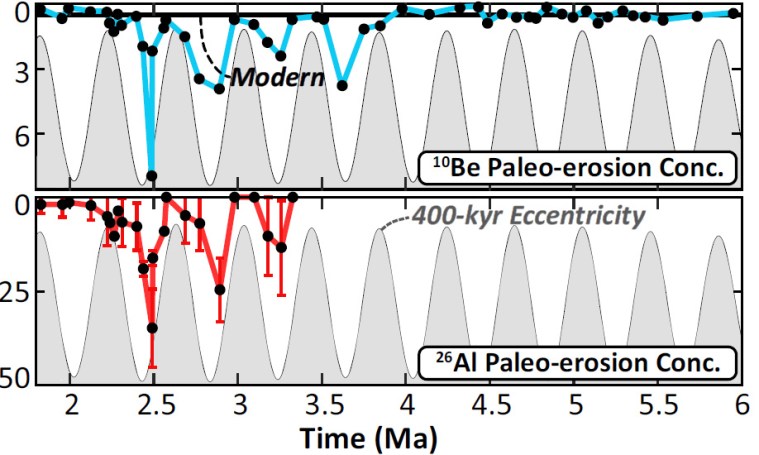
The data from 10Be suggest that erosion rates were consistently high from 6 to 4 Ma, but four times during the later Pliocene and the earliest Pleistocene they slowed dramatically. Each of these episodes occupies downturns in solar warming forced by the 400 ka cycle of orbital eccentricity. The 26Al record confirms this trend. The most likely reason for the slowing of erosion is long-term reductions in rainfall, which Fisher et al have modelled based on Milankovich cycles. However the modelled fluctuations are subtle, suggesting that in the Central Andes at least erosion rates were highly sensitive to climatic fluctuations. Yet the last 400 ka cycle in the record shows no apparent correlation with climate change.  Despite that, astronomical forcing while early Pleistocene oscillations between cooling and warming ramped up does seem to have affected erosion rates based on the cosmogenic dating. The authors attribute this loss of the 400 ka pattern to a kind of swamping effect of dramatically increased erosion rates as the regional climate became more erratic. Whether or not data of this kind will emerge for the more climatically drastic 100 ka cyclicity of the last million years remains to be seen … Anyone who has walked over terrains covered in glacial tills and glaciofluvial gravel beds nearer to the former Late Pleistocene ice sheets can judge the difficulty of such a task.

Early land plants and oceanic extinctions

In September 2022 Earth-logs highlighted how greening of the continents affected the composition of the continental crust. It now seems that was not the only profound change that the first land plants wrought on the Earth system. Beginning in the Silurian, the spread of vegetation swept across the continents during the Devonian Period. From a height of less than 30 cm among the earliest species by the Late Devonian the stature of plants went through a large increase with extensive forests of primitive tree-sized conifers, cycads, horsetails and sporiferous lycopods up to 10 m tall. Their rapid evolution and spread was not hampered by any herbivores. It was during the Devonian that tetrapod amphibians emerged from the seas, probably feeding on burgeoning terrestrial invertebrates. The Late Devonian was marked by five distinct episodes of extinction, two of which comprise the Devonian mass extinction: one of the ‘Big Five’. This affected both marine and terrestrial organisms. Neither flood volcanism nor extraterrestrial impact can be linked to the extinction episodes. Rather they marked a long drawn-out period of repeated environmental stress.

Phytoplankton bloom off the east coast of Scotland ‘fertilised’ by effluents carried by the Tay and Forth estuaries.

One possibility is that a side effect of the greening of the land was the release of massive amounts of nutrients to the seas that would have resulted in large-scale blooms of phytoplankton whose death and decay depleted oxygen levels in the water column. That is a process seen today where large amounts of commercial fertilisers end up in water bodies to result in their eutrophication. Matthew Smart and others from Indiana University-Purdue University, USA and the University of Southampton, UK, geochemically analysed Devonian lake deposits from Greenland and Scotland to test this hypothesis (Smart, M.S. et al. 2022. Enhanced terrestrial nutrient release during the Devonian emergence and expansion of forests: Evidence from lacustrine phosphorus and geochemical records. Geological Society of America Bulletin, v. 134, early release article;  DOI: 10.1130/B36384.1).

Smart et al. show that in the Middle and Late Devonian the lacustrine strata show cycles in their abundance of phosphorus (P an important plant nutrient) that parallel evidence for wet and dry cycles in the lacustrine basins. The cycles show that the same phosphorus abundance patterns occurred at roughly the same times at five separate sites. This may suggest a climatic control forced by changes in Earth’s orbital behaviour, similar to the Milankovich Effect on the Pleistocene climate and at other times in Phanerozoic history. The wet and dry intervals show up in the changing ratio between strontium and copper abundances (Sr/Cu): high values signify wet conditions, low suggesting dry. The wet periods show high ratios of rubidium to strontium (Rb/Sr) that suggest enhanced weathering, while dry periods show the reverse – decreased weathering.

When conditions were dry and weathering low, P built up in the lake sediments, whereas during wet conditions P decreases; i.e. it was exported from the lakes, presumably to the oceans. The authors interpret the changes in relation to the fate of plants under the different conditions. Dry periods would result in widespread death of plants and their rotting, which would release their P content to the shallowing, more stagnant lakes. When conditions were wetter root growth would have increased weathering and more rainfall would flush P from the now deeper and more active lake basins. The ultimate repository of the sediments and freshwater, the oceans, would therefore be subject to boom and bust (wet and dry) as regards nutrition and phytoplankton blooms. Dead phytoplankton, in turn, would use up dissolved oxygen during their decay. That would lead to oceanic anoxia, which also occurred in pulses during the Devonian, that may have contributed to animal extinction.

See also: Linking mass extinctions to the expansion and radiation of land plants, EurekaAlert 10 November 2022; Mass Extinctions May Have Been Driven by the Evolution of Tree Roots, SciTechDaily, 14 November 2022.

Milankovich precession and the Palaeocene-Eocene Thermal Maximum

About 56 Ma ago there occurred some of the most dramatic biological changes since the mass extinction at the Cretaceous-Palaeogene boundary. They included rapid expansion and diversification of mammals and land plants, and a plunge in the number of deep-water foraminifera. Global cooling from the Cretaceous hothouse was rudely reversed by sudden global warming of about 5 to 10°C. Some climatologists have ascribed bugbear status to the Palaeocene-Eocene Thermal Maximum (PETM) as a possible scenario for future anthropogenic global warming. The widely accepted cause is a massive blurt into the Palaeocene atmosphere of greenhouse gases, but what caused it is enthusiastically debated. The climate shift is associated with a sudden decrease in the proportion of 13C in marine sediments: a negative spike in δ13C. Because photosynthesis favours the lighter 12C, organic matter has a low δ13C, so a great deal of buried organic carbon may have escaped from the ocean floor, most likely in the form of methane gas. However, massive burning of living terrestrial biomass would produce the same carbon-isotope signal, but absence of evidence for mass conflagration supports methane release. Methane is temporarily held in marine sediments in the form of gas hydrate (clathrate), an ice-like solid that forms at low temperatures on the deep seafloor. Warming of deep sea water or a decrease in pressure, if sea level falls, destabilise clathrates thereby releasing methane gas: the ‘clathrate gun hypothesis’. The main issue is what mechanism may have pulled the trigger for a monstrous methane release.

Massive leak of natural gas – mainly methane – off Sweden in the Baltic Sea, from the probably sabotaged Nord Stream pipeline. (Source: Swedish coastguard agency)

Many have favoured a major igneous event. Between 55.0 and 55.8 Ma basaltic magmatism– continuing today in Iceland – formed the North Atlantic Igneous Province. It involved large-scale intrusion of sills as well as outpourings of flood basalts and coincided with the initial rifting of Greenland from northern Europe (see: Smoking gun for end-Palaeocene warming: an igneous connection; July/August 2004). The occurrence of impact ejecta in end-Palaeocene sediments off the east coast of the US has spawned an extraterrestrial hypothesis for the warming, which could account for the negative spike in δ13C as the product of a burning terrestrial biosphere (see: Impact linked to the Palaeocene-Eocene boundary event; October 2016). Less headline-grabbing is the possibility that the event was part and parcel of the Milankovich effect: an inevitability in the complex interplay between the three astronomical components that affect Earth’s orbital and rotational behaviour: eccentricity, axial tilt and precession. A group of geoscientists from China and the US, led by Mingsong Li of Peking University, have investigated in minute detail the ups and downs of δ13C around 56 Ma in drill cores recovered from a sequence of Palaeocene and Eocene continental-shelf sediments in Maryland, USA (Li, M., Bralower, T.J. et al. 2022. Astrochronology of the Paleocene-Eocene Thermal Maximum on the Atlantic Coastal Plain. Nature Communications, v. 13, Article 5618; DOI: 10.1038/s41467-022-33390-x).

The study involved sampling sediment for carbon- and oxygen-isotope analysis at depth intervals between 3 and 10 cm over a 35 m section through the lower Eocene and uppermost Palaeocene. Calcium abundances in the core were logged at a resolution of 5 mm using an X-ray fluorescence instrument. The results link to variations in CaCO3 in the sediments across the PETM event. Another dataset involves semi-continuous measurements of magnetic susceptibility (MS) along the core. These measurements are able to indicate variations in delivery to the ocean of dissolved calcium and detrital magnetic minerals as climate and continental weathering vary through time. They are widely known to be good recorders of Milankovich cycles. After processing, the Ca and MS data sets show cyclical fluctuations relative to depth within the cores. ‘Tuning’ their frequencies to the familiar time series of Milankovich astronomical climate forcing reveals a close match to what would be expected if the climate fluctuations were paced by the 26 ka axial precession signal. My post of 17 June 2022 about the influence of precession over ‘iceberg armadas’ during the Pleistocene might be useful to re-read in this context. This correlation enabled the researchers to convert depth in the cores to time, so that the timing of fluctuations in carbon- and oxygen-isotope data that the PETM had created could be considered against various hypotheses for its cause. The ‘excursions’ of both began at the same time and reached the maxima of their changes from Palaeocene values over about 6,000 years. The authors consider that is far too long to countenance the release of methane as a result of asteroidal impact, or by massive burning of terrestrial vegetation. The other option that the beginning of the North Atlantic Igneous Province had been the trigger may also be ruled out on two grounds: the magmatism began earlier, and it continued for far longer. The onset of the PETM coincides with an extreme in precession-related climatic forcing. So Li et al. consider that a quirk in the Milankovich Effect could have played a role in triggering massive methane release. This might also explain features of the global calcium record in seafloor sediments as results of a brief period of ocean acidification during the PETM. Such an event would play havoc with carbonate-secreting organisms, such as foraminifera, by lowering the dissolved carbonate ion content on which they depend for their shells: hence their suffering considerable extinction. Of course, the other elements of astronomical forcing – eccentricity and axial tilt – would also have been operating on global climate at the time.  The long-term 100 and 405 ka eccentricity cycles may have played a role in amplifying warming, which may have resulted in increased burial of organic carbon and thus the amount of methane buried beneath the seabed.

A new twist to Pleistocene climate cycles

The combined gravitational pulls of the sun and moon modulate variations in local tidal range. High spring tides occur when the two bodies are opposed at full moon or in roughly the same direction at new Moon. When the positions of sun and moon are at right angles (1st quarter and 3rd quarter) their gravitational pulls partly cancel each other to give neap tides. Consequently, there are two tidal cycles every lunar month.  In a similar way, the varying gravitational pulls of the planets during their orbital cycles impart a repetitive harmony to Earths astronomical behaviour. But their combined effects are on the order of tens of thousand years. Milutin Milankovich (1879-1958), a Serbian engineer, pondered on the possible causes of Earth’s climatic variations, particularly the repetition of ice ages. He was inspired by 19th century astronomers’ suggestion that maybe the gravitational effects of other planets might be a fruitful line of research. Milankovich focussed on how the shape of Earth’s orbit, the tilt of its rotational axis and the way the axis wobbles like that of a spinning top affect the amount of solar heating at all points on the surface: the effects of varying eccentricity, obliquity and precession, respectively.

 Earlier astronomers had calculated cycles of gravitational effects on Earth of the orbits of Jupiter and Saturn of the three attributes of Earth’s astronomical behaviour and found periods of about 100, 41 and 23 thousand years (ka) respectively. The other 3 inner planets and the much more distant giants Uranus and Neptune also have gravitational effects on Earth, but they are negligible compared with those of the two nearest giant planets, because gravitation force varies with mass and inversely with the square of distance. Sadly, Milankovich was long dead when his hypothesis of astronomical climate forcing was verified in 1976 by frequency analysis of the record of oxygen isotopes in foraminifera found in two ocean sediment core from the Southern Indian Ocean. It revealed that all three periods interfered in complex ways during the Late Pleistocene, to dominate variations in sea-surface temperatures and the fluctuating volume of continental ice sheets for which δ18O is a proxy (see: Odds and ends about Milankovich and climate change; February 2017).

Precession of the axis of a spinning top and that of the Earth. At present the northern end of Earth’s axis points to what we now call the Pole Star. Around 11.5 ka from now it will point to the star Vega

This was as revolutionary for climatology as plate tectonics was for geology. We now know that in the early Pleistocene glacial-interglacial cycles were in lockstep with the 41 ka period of axial obliquity, and since 700 ka followed closely – but not perfectly – the 100 ka orbital eccentricity forcing. The transitional period between 1.25 and 0.7 Ma (the Mid-Pleistocene Transition or MPT) suggested neither one nor the other. Milankovich established that axial tilt variations have the greatest influence on solar heating, so the early 41 ka cycles were no surprise. But the dominance of orbital eccentricity on the last 700 ka certainly presented a puzzle, for it has by far the weakest influence on solar heating: 10 times less than those of axial obliquity and precession. The other oddity concerns the actual effect of axial precession on climate change. There are no obvious 23 ka cycles in the climate record, despite the precession signal being clear in frequency analysis and its effect on solar heating being almost as powerful as obliquity and ten times greater than that of orbital eccentricity. Precessional wobbling of the axis controls the time of year when one hemisphere or the other is closest to the Sun. At one extreme it will be the Northern and 11.5 ka later it will be the Southern. The times of solstices and equinoxes also change relative to the calendar that we use today.

There is an important, if obvious, point about astronomical forcing of climate. It is always there, with much the same complicated interactions between the factors: human activities have absolutely no bearing on them. Climatic ‘surprises’ are likely to continue!

Changes in ice-rafted debris (IRD) since 1.7 Ma in a sediment core from the North Atlantic (orange fill) compared with its oxygen-isotope (δ18O) record of changes in continental ice cover (blue fill). At the top are the modelled variations in 23 ka axial precession (lilac) and 41 ka obliquity (green). The red circles mark major interglacial episodes, blue diamonds show the onset of significant ice rafting and orange diamonds are terminations of ice-rafting (TIR). (Credit: Barker et al., Fig. 2)

Sea temperature and ice-sheet volume are not the only things that changed during the Pleistocene. Another kind of record from oceanic sediments concerns the varying proportion in the muddy layers of abnormally coarse sand grains and even small pebbles that have been carried by icebergs; they are known as ice-rafted debris (IRD). The North Atlantic Ocean floor has plenty of evidence for them appearing and disappearing on a layer-by-layer basis. They were first recognised in 1988 by an oceanographer called Helmut Heinrich, who proposed that six major layers rich in IRD in North Atlantic cores bear witness to iceberg ‘armadas’ launched by collapse, or ablation, at the front of surging ice sheets on Scandinavia, Greenland and eastern Canada. Heinrich events, along with Dansgaard-Oeschger events (rapid climatic warming followed by slower cooling) in the progression to the last glacial maximum have been ascribed to a variety of processes  operating on a ‘millennial’ scale. However, ocean-floor sediment cores are full of lesser fluctuations in IRD, back to at least 1.7 Ma ago. That record offers a better chance of explaining fluctuations in ice-sheet ablation. A joint European-US group has investigated their potential over the last decade or so (Barker, S. et al. 2022. Persistent influence of precession on northern ice sheet variability since the early Pleistocene. Science, v. 376, p. 961-967; DOI: 10.1126/science.abm4033). The authors noted that in each glacial cycle since 1.7 Ma the start of ice rafting consistently occurred during a time of decreasing axial obliquity. Yet the largest ablation events were linked to minima in the precession cycles. In the last 700 ka, such extreme events are associated with the terminations of each ice age.

In the earlier part of the record, the 41 ka obliquity ‘signal’ was sufficient to drive glacial-interglacial cycles, hence their much greater regularity and symmetry than those that followed the Mid-Pleistocene Transition. The earlier ice sheets in the Northern Hemisphere also had consistently smaller extents than those after the MPT. Although the records show a role for precession in pre-MPT times in the form of ice-rafting events, the lesser effect of precession on summer warming at higher latitudes, compared with that of axial obliquity, gave it no decisive influence. After 700 ka the northern ice sheets extended much further south – as far as 40°N in North America – where summer warming would always have been commensurately greater than at high northern latitudes. So they were more susceptible to melting during the increased summer warming driven by the precession cycles. When maximum summer heating induced by axial precession in the Northern Hemisphere coincided with that of obliquity the ice sheets as a whole would have become prone to catastrophic collapse.

It is hard to say whether these revelations have a bearing on future climate. Of course, astronomical forcing will continue relentlessly, irrespective of anthropogenic greenhouse gas emissions. Earth has been in an interglacial for the last 11.5 ka, since the Younger Dryas; i.e. about half a precession cycle ago. The combination of obliquity- and precession-driven influences suggest that climate should be cooling and has been since 6,000 years ago, until the Industrial Revolution intervened. Can the gravitational pull of the giant planets prevent a runaway greenhouse effect, or will human effects defy astronomical forces that continually distort Earth’s astronomical behaviour?

Signs of Milankovich Effect during Snowball Earth episodes

The idea that the Earth was like a giant snowball during the Neoproterozoic Era arose from the discovery of rocks of that age that could only have formed as a result of glaciation. However, unlike the Pleistocene ice ages, evidence for these much older glacial conditions occurs on all continents. In some locations remanent magnetism in sedimentary rocks of that age is almost horizontal; i.e. they had been deposited at low magnetic latitudes, equivalent to the tropics of the present day. Frigid as it then was, the Earth still received solar heating and magmatic activity would have been slowly adding CO2 to the atmosphere so that less heat escaped – a greenhouse effect must have been functioning. Moreover, an iced-over world would not have been supporting much photosynthetic life to draw down the greenhouse gas into solid carbohydrates and carbonates to be buried on the ocean floor. As far as we know the Solar System’s geometry during the Neoproterozoic was much as it is today. So changes in the gravitational fields induced by the orbiting Giant Planets would have been affecting the shape (eccentricity) of Earth’s orbit, the tilt (obliquity) of its rotational axis and the precession (wobble) of its rotation as they do at present through the Milankovich effect. These astronomical forcings vary the amount of solar energy reaching the Earth’s surface. It has been suggested that a Snowball Earth’s climate system would have been just as sensitive to astronomical forcing as it has been during the last 2 million years or more. Proof of that hypothesis has recently been achieved, at least for one of the Snowball events (Mitchell, R.N. and 8 others 2021. Orbital forcing of ice sheets during snowball Earth. Nature Communications, v. 12, article 4187; DOI: 10.1038/s41467-021-24439-4).

Another of the enigmas of the Neoproterozoic is that after and absence of more than a billion years banded iron formations (see: Banded iron formations (BIFs) reviewed, December 2017) began to form again. BIFs are part of the suite of sedimentary rocks that characterise Snowball Earth events, often alternating with glaciogenic sediments. Throughout each cold cycle – the Sturtian (717 to 663 Ma) and Marinoan (650 to 632 Ma) glacial periods – conditions of sediment deposition varied a great deal from place to place and over time. Some sort of cyclicity is hinted at, but the pace of alternations has proved impossible to check, partly because the dominant rocks (glacial conglomerates or diamictites) show little stratification and others that are bedded (various non-glacial sandstones) vary from place to place and give no sign of rates of deposition, having been deposited under high-energy conditions. BIFs, on the other hand are made up of enormous numbers of parallel layers on scales from millimetres to centimetres. Bundles of bands can be traced over large areas, and they may represent repeated cycles of deposition.

Typical banded iron formation

How BIFs formed is crucial. They were precipitated from water rich in dissolved iron in its reduced Fe2+ (ferrous) form, which originated from sea-floor hydrothermal vents. Precipitation occurred when the amount of oxygen in the water increased the chance of electrons being removed from iron ions to transform them from ferrous to ferric (Fe3+). Their combination with oxygen yields insoluble iron oxides. Cyclical changes in the availability of oxygen and the balance between reducing and oxidising conditions result in the banding. In fact several rhythms of alternation are witnessed by repeated packages at deci-, centi- and millimetre scales within each BIF deposit. Overall the packages suggest a constant rate of deposition: a ‘must-have’ for precise time-analysis of the cycles. BIFs contain both weakly magnetic hematite (Fe2O3) and strongly magnetic magnetite (Fe3O4), their ratio depending on varying geochemical conditions during deposition. Ross Mitchell of Curtin University, Western Australia and his Chinese, Australian and Dutch colleagues measured magnetic susceptibility at closely spaced intervals (1 and 0.25 m) in two section of BIFs from the Sturtian glaciation in the Flinders Ranges of South Australia. Visually both sections show clear signs of two high-frequency and three lower frequency kinds of cycles, expressed in thickness.

The tricky step was converting the magneto-stratigraphic data to a time series. High-precision zircon U-Pb dating of volcanic rocks in the sequence suggested a mean BIF deposition rate of 3.7 to 4.4 cm per thousand years. This allowed the thickness of individual bands and packages to be expressed in years, the prerequisite for time-series analysis of the BIF magneto-stratigraphic sequence. This involves a mathematical process known as the Fast-Fourier Transform, which expresses the actual data as a spectral curve. Peaks in the curve represent specific frequencies expressed as cycles per metre. The rate of deposition of the BIF allows each peak to be assigned a frequency in years, which can then be compared with the hypothetical spectrum associated with the Milankovich effect. One of the BIF sequences yielded peaks corresponding to 23, 97 and 106 ka. These match the effects of variation in precession (23 ka) and ‘short’ orbital eccentricity (97 and 106 ka) found in Cenozoic sea-floor sediments and ice cores. The other showed peaks at 405, 754 and 1.2 Ma corresponding to ‘long’ orbital eccentricity and long-term features of both obliquity and precession. Quite a result! But how does this bear on Snowball Earth events? Cyclical changes in solar heating would have affected the extent of ice sheets and sea ice at all latitudes, forcing episodes of expansion and contraction and thus changes in sediment supply to the sea floor. That helps explain the many observed variations in sedimentation other than that of BIFs. Rather than supporting a ‘hard’ Snowball model of total marine ice cover for millions of years, it suggests that such an extreme was relieved by period of extensive open water, much as affected the modern Arctic Ocean for the last 2 million years or so. There could have been global equivalents of ice ages and interglacials during the Sturtian and Marinoan. ‘Hard’ conditions would have shut down much of the oceans’ biological productivity, periodically to have been reprieved by more open conditions: a mechanism that would have promoted both extinctions and evolutionary radiations. Snowball events may have driven the takeover of prokaryote (bacteria) dominance by that of the multicelled eukaryotes that is signalled by the Ediacaran faunas that swiftly followed glacial epochs and the explosion of multicelled life during the Cambrian. As eukaryotes, we may well owe our existence to Snowball.

Very persistent cycles

Carboniferous shale
Carboniferous shale (Photo credit: tehsma)

The last of five written papers in my 1967 final-year exams was, as always, set by the ‘Prof’.  One question was ‘Rock and rhythm: discuss’ – it was the 60s. Cyclicity has been central to observational geology, especially to stratigraphy, the difference from that era being that rhythms have been quantified and the rock sequences they repeat have been linked to processes, in many cases global ones. The most familiar cyclicity to geologists brought up in Carboniferous coalfields, or indeed any area that preserves Carboniferous marine and terrestrial rocks, is the cyclothem of, roughly, seat-earth – coal – marine shale – fluviatile sandstone – seat-earth and so on. Matched to the duration of Carboniferous to Permian glaciations of the then southern hemisphere, and with the relatively  new realisation that global sea level goes down  and up as ice caps wax and wane, the likeliest explanation is eustatic regression and transgression of marine conditions in coastal areas in response to global climate change. Statistical analysis of cyclothemic sequences unearths frequency patterns that match well those of astronomical climate forcing proved for Pleistocene glacial-interglacial cycles.

The Milankovich signals of the Carboniferous are now part of the geological canon, but rocks of that age more finely layered than sediments of the tropical continental margins do occur. Among them are rhythmic sequences interpreted as lake deposits from high latitudes, akin to varves formed in such environments nowadays. Those from south-western Brazil present spectacular evidence of climate change in the Late Carboniferous and Early Permian (Franco, D.R. et al. 2012. Millennial-scale climate cycles in Permian-Carboniferous rhythmites: Permanent feature throughout geological time. Geology, v. 40, p. 19-22). They comprise couplets of fine-grained grey quartz sandstones from 1-10 cm thick interleaved with black mudstones on a scale of millimetres, which together build up around 45 m of sediment. Their remanent magnetism and magnetic susceptibility vary systematically with the two components. Frequency analysis of plots of both against depth in the sequence show clear signs of regular repetitions. Low-frequency peaks reveal the now well-known influence of astronomical forcing of Upper Palaeozoic climate, but it is in the lower amplitude, higher frequency part of the magnetic spectrum that surprises emerge from a variety of peaks. They are reminiscent of the Dansgaard-Oeschger events of the last Pleistocene glacial, marked by sudden warming and slow cooling while world climate cooled towards the last glacial maximum (~1.5 ka cyclicity) and Heinrich events, the ‘iceberg armadas’ that occurred on a less regular 3 to 8 ka basis. There are also signs of the 2.4 ka solar cycle. The relatively brief cycles would have been due to events in a very different continental configuration from today’s – that of the supercontinent Pangaea – and their very presence suggests a more general global influence over short-term climate shifts that has been around for 300 Ma or more.

OSTM/Jason-2's predecessor TOPEX/Poseidon caug...
El Niño effect on sea -surface temperatures in the eastern Pacific Ocean. Image via Wikipedia

Closer to us in time, and on a much finer time scale are almost 100 m of finely laminated shales from the marine Late Cretaceous of California’s Great Valley (Davies, A. et al. 2012. El Niño-Southern Oscillation variability from the late Cretaceous Marca Shale of California. Geology, v. 40, p. 15-18). The laminations contain fossil diatoms: organisms that are highly sensitive to environmental conditions and whose species are easily distinguished from each other. It emerges from studies of the diatoms in each lamination set that they record an annual cycle of seasonal change related to marine upwellings and their varying strengths, with repeated evidence for influx of fine sediment derived from land above sea level and for varying degrees of bioturbation that suggests periods of oxygenation. Spectral analysis of the intensity of bioturbation, which assumes the lamina are annual, and other fluctuating features reveals peaks that are remarkably close to those of the ENSO cyclicity that operates at present, at 2.1-2.8 and 4.1-6.3 a, as well as repetitions with a decadal frequency.

The annual cycles bear similar hallmarks to those imposed by the monsoonal conditions familiar from modern California, which fluctuated in the Late Cretaceous in much the same way as it does now – roughly speaking, alternating El Niño and La Niña conditions. That is not so surprising, as the relationship between California and the Pacific Ocean in the Cretaceous would not have been dissimilar from that now. The real importance of the study is that it concerns a period in Earth’s climate history characterised by greenhouse conditions, that some predict would create a permanent El Niño – an abnormal warming of surface ocean waters in the eastern tropical Pacific that prevents the cold Humboldt Current along the Andean coast of South America from supplying nutrient to tropical waters. The very cyclicity recorded by the Marca Shale strongly suggests that the ENSO is a stable feature of the western Americas. Recent clear implications of ENSO having teleconnections that affect global climate, on this evidence, may not break down with anthropogenic global warming. This confirms similar studies from the Palaeogene and Neogene Periods.