How humans might have migrated into the Americas

When and how humans first migrated into the Americas are issues that have exercised anthropologists for the last two decades, often sparking off acrimonious debate. In the 20th century both seemed to well established: hunters using the celebrated Clovis fluted spear blades arrived first, no earlier than 13 ka ago. The Beringia land bridge across what is now the Bering Strait was exposed by falling sea level as early as 30 thousand years ago in the lead-up to the last glacial maximum (LGM) to link eastern Siberia and Alaska. However, ice sheets expanding to the south-west of the main area of glaciation on the Canadian Shield barred passage through Interior Alaska and NW Canada. Only around 13 ka had a N-S ice-free corridor opened through the mountains during glacial retreat. Nevertheless, humans had entered Alaska at least ten thousand years earlier, during the LGM, to occupy caves in its western extremity: Alaska was habitable but they were stuck there.

In the early 21st century, it became clear that the ‘Clovis First’ hypothesis was mistaken. Sediments in Texas that contained Clovis blades were found to be underlain by those of an older culture, reliably dated to about 15.5 ka. Furthermore, analysis of the DNA of all groups of native Americans (north and south) indicated a last common ancestor in Siberia more than 30 ka ago: they descended from that ancestor outside of Asia. More recently excavated sites in Mexico and Chile point to human populations having reached there as early at 33 ka (see: Earliest Americans, and plenty of them; July 2020), and there is a host of pre-Clovis sites in North and Central America dating back to 18.2 ka. Such ancient groups could not have walked from the Beringia land bridge because the present topographic grain in the Western Cordillera would have been blocked by ice since about 25 thousand years ago. The only viable possibility was that they followed the Alaskan coast to move southwards, either in boats or over sea ice.
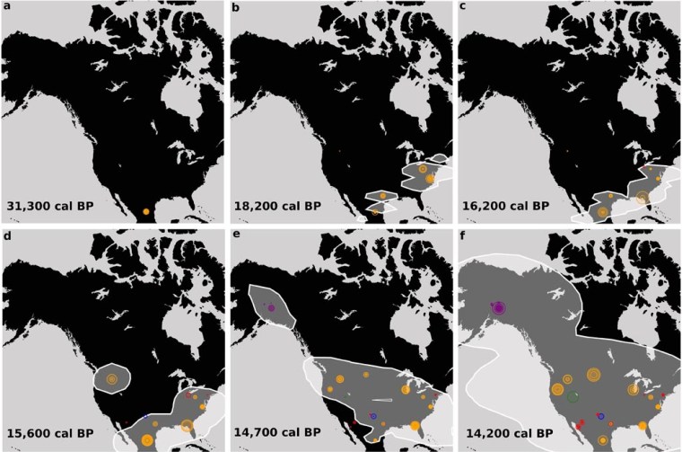
Dated pre-Clovis sites in Mexico and North America and possible expanding distribution of people from 31.3 to 14.2 ka (Credit; Becerra-Valdivia and Higham; Extended Data Fig. 4)

A new focus on when such journeys would have been feasible was published in February 2023 (Praetorius, S.K et al. 2023. Ice and ocean constraints on early human migrations into North America along the Pacific coast. Proceedings of the National Academy of Science, v. 120, article e2208738120; DOI: 10.1073/pnas.2208738120). One advantage of moving along the coast is that, though it would be pretty cold, the warming effect of the Pacific Ocean would make it more bearable than travelling inland, where winter temperatures even today regularly reach -50°C. More important, there would be no shortage of food; fish, marine mammals and shellfish abound at the ice margin or onshore, at any season. But a coastal route may not have been possible at all times during the period either side of the LGM. Large glaciers still reach the ocean from Alaska and there is little more perilous than crossing the huge crevasse fields that they present. Boating would have been highly dangerous because of continual calving of icebergs from extensive ice shelves. Moreover, the Alaska Coastal Current flows northwards and would likely have sped up during episodes of glacial melting as the current is affected by fresh water influx. Yet there may sometimes have been episodes of open water at the ice front frozen to relatively flat sea ice in winter. That would making boat- or foot travel relatively safe. Sea ice would also make glacier-free islands accessible for encampments over the harsh winters or even for hundreds of years, with plenty of marine food resources.

Summer Praetorius of the US Geological Survey and colleagues from Woods Hole Oceanographic Institution, Oregon State University, and the Universities of California (Santa Cruz) and Oregon have attempted to model conditions since 32.5 ka ago in coastal waters off Northwest America. They used simulations of the behaviour of the Alaska Coastal Current during varying climate conditions before and during the LGM, while glaciers were in  retreat that followed and during the Holocene. Their modelling is based on the effects of changing sea level and water salinity on general circulation in the Northern Pacific. The relative abundance of sea ice can be tracked using variation in an alkenone produced by phytoplankton that wax and wane according to sea-surface temperature and sea-ice cover. The other input is the well-documented changing extent of continental glaciation in Alaska and the Yukon Territory. Based on their model they estimate that the most favourable environmental conditions for coastal migration occurred just before the LGM (24.5 to 22 ka) and between 16.4 and 14.8 ka during the initial stages of warming and extensive melting of ice sheets. The Alaskan Coastal Current probably doubled in intensity during the LGM making the use of boats highly dangerous

By 35 ka ocean-going boats are known to have been used by people in northern Japan. Traversing sea-ice was the way in which Inuit people occupied all the Arctic coastal areas of North America and Greenland during the last five thousand years, and is the form of travel favoured by the authors. It is not yet possible to prove and date such coastal journeys because campsites or settlements along the coast would now be inundated by 100 m of post-glacial sea-level rise. Yet such migration was necessary to establish settlements at lower latitudes in North America and Mexico in the period when overland routes from Beringia were blocked by ice sheets. By 32.5 ka falling sea level probably made it possible to cross the Bering Strait for the first time and for the next 7.5 ka an ice-free corridor made it possible for the rest of North America and points further south to be reached on-foot from Alaska. That window of opportunity might have allowed humans to have reached Mexico and South America, where the earliest dates of occupation have been found. But many of the early sites across North America date to the period (25 to 13 ka) when overland access was blocked. Of course, those sites might have been established by expansion from the very earliest migrants who crossed the Beringia land bridge and took advantage of overland passage before 25 ka. But if later migrants from Asia could follow the coastal route, then it seems likely that they did. Later Inuit spread along  the shores of the Arctic Ocean since 5000 years ago probably with a material culture little different from that of the earlier migrants from Siberia.

Naturally occurring hydrogen: an abundant green fuel?

Burning hydrogen produces only water vapour, so it is not surprising that it has been touted as the ultimate ‘green’ energy source, and increasingly attracts the view that the ‘Hydrogen Economy’ may replace that based on fossil fuels. It is currently produced from natural gas by ‘steam reforming’ of methane that transforms water vapour and CH4 to hydrogen and carbon monoxide. That clearly doesn’t make use of the hydrogen ‘green’ as the CO becomes carbon dioxide because it reacts with atmospheric oxygen; it is termed ‘grey hydrogen’. But should it prove possible to capture CO and store it permanently underground in some way then that can be touted as ‘blue hydrogen’ thereby covering up the carbon footprint of all the rigmarole in getting the waste CO into a safe reservoir. However, if carbon-free electricity from renewables is used to electrolyse water into H and O the hydrogen aficionados can safely call it ‘green hydrogen’.   It seem there is a bewildering colour coding for hydrogen that depends on the various options for its production: ‘yellow’ if produced using solar energy; ‘red’ if made chemically from biowaste; ‘black’ by coking coal using steam; ‘pink’ is electrolysis using nuclear power; and even ‘turquoise’ hydrogen if methane is somehow turned into hydrogen and solid carbon using renewables – a yet-to-be-developed technology! Very jolly but confusing: almost suspiciously so!

But not to be forgotten is the ‘white’ variety, applied to hydrogen that is emitted by natural processes within the Earth. Eric Hand, the European news editor for the major journal Science has written an excellent Feature article about ‘white’ hydrogen in a recent issue (Hand, E. 2023. Hidden hydrogen. Science, v. 379, article adh1460; DOI: 10.1126/science.adh1460). Hand’s feature is quirky, but well-worth a read. It is based on the proceedings of a Geological Society of America mini-conference about non-petroleum, geological energy resources  held in October 2022. He opens with a bizarre anecdote related by a farmer who lives in rural Mali. The only drilling that ever went on in his village was for water, and many holes were dry. But one attempt resulted in ‘wind coming out of the hole’. When a driller looked in the hole, the ‘wind’ burst into flame – he had a cigarette in his mouth. The fire burned for months. Some 20 years later the story reached a Malian company executive who began prospecting the area’s petroleum potential, believing the drilling had hit natural gas. Analysis of the gas revealed that it was 98% hydrogen – now the village has electricity generated by ‘white’ hydrogen.

Mantle rock in the Oman ophiolite, showing cores of fresh peridotite, surrounded by brownish serpentinite and white magnesium carbonate veins (credit: Juerg Matter, Oman Drilling Project, Southampton University, UK)

So how is hydrogen produced by geological processes? Some springs in the mountains of Oman also release copious amounts of the gas. The springs emerge from ultramafic rocks of the vast ophiolite that was emplaced onto the Arabian continental crust towards the end of the Cretaceous. The lower part of this obducted mass of oceanic lithosphere is mantle rock dominated by iron- and magnesium-rich silicates, mainly olivine [(Mg,Fe)2SiO4 – a solid solution of magnesium and iron end members]. When saturated with groundwater in which CO2 is dissolved olivine breaks down slowly but relentlessly. The hydration reaction is exothermic and generates heat, so is self-sustaining. Olivine’s magnesium end member is hydrated to form the soft ornamental mineral serpentine (Mg3Si2O5(OH)4) and magnesium carbonate. Under reducing conditions the iron end member reacts with water to produce an iron oxide, silica and hydrogen:

3Fe2SiO4 + 2H2O → 2 Fe3O4 + 3SiO­2 +3H2

Gases emanating from mid-ocean ridges contain high amounts of hydrogen produced in this way, for example from Icelandic geothermal wells. But Mali is part of an ancient craton, so similar reactions involving iron-rich ultramafic rocks deep in the continental crust are probably sourcing hydrogen in this way too. Hydrogen production on the scale of that discovered in Mali seems to be widespread, with discoveries in Australia, the US, Brazil and the Spanish Pyrenees that have pilot-scale production plants. The US Geological Survey has estimated that around 1 trillion tonnes of ‘white’ hydrogen may be available for extraction and use

Hydrogen, like other natural gases, may be trapped below the surface in the same ways as in commercial petroleum fields. But petroleum-gas wells emit little if any hydrogen mixed in with methane. That absence is probably because petroleum fields occur in deep sedimentary basins well above any crystalline basement. The geophysical exploration that discovers and defines the traps in petroleum fields has never been deployed over areas of crystalline continental crust because as far as the oil companies are concerned they are barren. That may be about to change. There is another exploration approach: known hydrogen seepage seems to deter vegetation so that the sites are in areas of bare ground, which have been called ‘fairy circles’. These could be detected easily using remote sensing techniques.

Artificially increasing serpentine formation by pumping water into the mantle part of ophiolites, such as that in Oman, and other near-surface ultramafic rocks is also a means of carbon sequestration, which should produce hydrogen as a by-product (see: Global warming: Can mantle rocks reduce the greenhouse effect?, July 2021). A ‘two-for-the-price-of-one’ opportunity?

Who invented stone tools? A great surprise from Kenya

Up to now the earliest stone tools are objects dated to about 3.3 Ma (Late Pliocene) found in the Turkana basin of Kenya in 2015. They are sharp-edged pieces of rock that seem to have been made simply by striking two lumps of rock together (see: Stone tools go even further back; May 2015). These Lomekwian artefacts are similar to the basic tools made today by some chimpanzees in parts of Africa. Their age matches that for the earliest known animal bones that show signs of having meat cut from them, which were unearthed in Dikika, Ethiopia (see: Another big surprise; September 2010) which, like the Lomekwian tools, are not accompanied by tools or hominin remains. The earliest tools associated with members of the genus Homo are significantly more sophisticated. They were found in close association with H. habilis at what seems to have been a well-used butchering site, dated at 2.0 Ma, in Tanzania’s Olduvai Gorge, hence their designation as the Oldowan ‘industry’. The Oldowan ‘tool kit’ includes choppers and blades deliberately shaped to be wielded by hand and made by striking large cobbles with distinctive hammer stones. Earlier tools with this level of deliberate crafting come from the 2.6 Ma Ledi-Geraru site in the Afar Depression of NE Ethiopia but with no sign of their makers.

Oldowan tools used for pounding and cutting from Nyayanga, Kenya (Credit: Thomas Plummer, James Oliver and Emma Finestone/Homa Peninsula Paleoanthropology Project/SWNS)

The presence of Oldowan tools has now been pushed further back, by about 400 ka, thanks to excavations in Late Pliocene sediments at Nyayanga on the shore of Lake Victoria in western Kenya by Thomas Plummer of Queens College in New York State, USA, and his numerous collaborators from the US, Germany, the UK, China, Italy, Australia, Kenya, South Africa and Poland (Plummer, T.W. and 31 others 2023. Expanded geographic distribution and dietary strategies of the earliest Oldowan hominins and Paranthropus. Science, v. 379, p. 561-566; DOI: 10.1126/science.abo7452). Their work also expands the range of Oldowan culture by about 1300 km. The Nyayanga site yielded over 300 artefacts that closely resemble the previously known range of Oldowan tool shapes. Their makers struck flakes from suitable corestones – made of rhyolite, quartz and quartzite – and trimmed them by more intricate means. They seem to have been used to cut up mainly hippo and buffalo, bones of which bear clear cut marks, but had other uses. Analysis of the wear on tool surfaces not only show signs of butchery, but also processing of plant tissue by pounding; the latter resulted in pitting and polishing of tools that seem to have been used many times. Stable-isotope analysis of the bones and animal teeth suggests that in the Pliocene Nyayanga was a grassy and partly wooded savannah close to a substantial water body needed by hippos.

Reconstruction of a Paranthropus head (Credit: Jerry Humphrey, Pinterest)

The ‘great surprise’ is that the only hominin remains associated with the site are two damaged molar teeth. They are so large that their most likely source was a species of Paranthropus.Paranthropoids have long been considered to be a gorilla-like, ‘robust’ branch of australopithecines. Their large cranial crests anchoring jaw muscles and enormous teeth were reckoned to indicate a diet of tough vegetation – the discoverer of the first specimen of P. boisei dubbed it ‘Nutcracker Man’ – although the wear on individual teeth suggests otherwise. But there is no reason to suppose that they could not eat meat. They survived australopithecines by more than a million years to cohabit the East African savannahs with H. ergaster until about 1 Ma ago.

Lead author Thomas Plummer wonders if paranthropoids would have needed tools because they had the largest jaws and teeth of any hominin. But had his team found close association with smaller H.habilis teeth would he have held a similarly negative view? There is evidence from younger sites in South Africa that paranthropoids used a wide diversity of bone tools and may even have been among the earliest fire users. So why the negativity about stone tools? To paraphrase Ali G, ‘Is it because they is ugly?’

See also: Devlin, H, Discovery of 3m-year-old stone tools sparks prehistoric whodunit. The Guardian, 9 February 2023

Is erosion paced by Milankovich cycles?

Both physical and chemical weathering reflects climatic controls. Erosion is effectively climate in continuous action on the Earth’s solid surface through water, air and bodies of ice moving under the influence of gravity. These two major processes on the land surface are immensely complicated. Being the surface part of the rock cycle, they interact with biological processes in the continents’ web of climate-controlled ecosystems. It is self-evident that climate exerts a powerful influence on all terrestrial landforms. But at any place on the Earth’s surface climate changes on a whole spectrum of rates and time scales as reflected by palaeoclimatology. With little room for doubt, so too do weathering and erosion. Yet other forces are at play in the development of landforms. ‘Wearing-down’ of elevated areas removes part of the load that the lithosphere bears, so that the surface rises in deeply eroded terrains. Solids removed as sediments depress the lithosphere where they are deposited in great sedimentary basins. In both cases the lithosphere rises and falls to maintain isostatic balance. On the grandest of scales, plate tectonics operates continuously as well. Its lateral motions force up mountain belts and volcanic chains, and drag apart the lithosphere, events that in themselves change climate at regional levels. Tectonics thereby creates ‘blips’ in long term global climate change. So evidence for links between landform evolution and palaeoclimate is notoriously difficult to pin down, let alone analyse.

The evidence for climate change over the last few million years is astonishingly detailed; so much so that it is possible to detect major global events that took as little as a few decades, such as the Younger Dryas, especially using data from ice cores. The record from ocean-floor sediments is good for changes over hundreds to thousands of years. The triumph of palaeoclimatology is that the last 2.5 Ma of Earth’s history has been proved to have been largely paced by variations in the Earth’s orbit and in the angle of tilt and wobbles of its rotational axis: a topic that Earth-logs has tracked since the start of the 21st century. The record also hints at processes influencing global climate that stem from various processes in the Earth system itself, at irregular but roughly millennial scales. The same cannot be said for the geological record of erosion, for a variety of reasons, foremost being that erosion and sediment transport are rarely continuous in any one place and it is more difficult to date the sedimentary products of erosion than ice cores and laminations in ocean-floor sediments. Nonetheless, a team from the US, Germany, the Netherlands , France and Argentina have tackled this thorny issue on the eastern side of the Andes in Argentina (Fisher, G.B. and 11 others 2023. Milankovitch-paced erosion in the southern Central Andes. Nature Communications, v. 14, 424-439; DOI: 10.1038/s41467-023-36022-0.

Burch Fisher (University of Texas at Austin, USA) and colleagues studied sediments derived from a catchment that drains the Puna Plateau that together with the Altiplano forms the axis of the Central Andes. In the late 19th century the upper reaches of the Rio Iruya were rerouted, which has resulted in its cutting a 100 m deep canyon through Pliocene to Early Pleistocene (6.0 to 1.8 Ma) sediments. The section includes six volcanic ash beds (dated precisely using the zircon U-Pb method) and records nine palaeomagnetic reversals, which together helped to calibrate more closely spaced dating. Their detailed survey used the decay of radioactive isotopes of beryllium and aluminium (10Be and 26Al) in quartz grains that form in the mineral when exposed at the surface to cosmic-ray bombardment. Such cosmogenic radionuclide dating thus records the last time different sediment levels were at the surface, presumably when the sediment was buried, and thus the variation in the rate of sediment supply from erosion of the Rio Iruya catchment since 6 Ma ago.

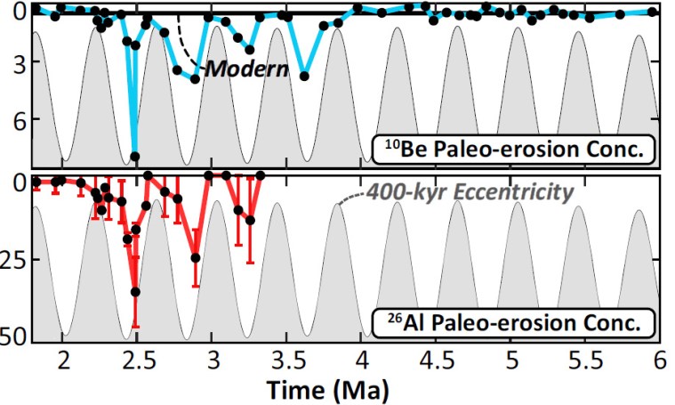
Measured concentrations (low to high values downwards) of cosmogenic 10Be (turquoise) and 26Al (red) in samples from the Rio Iruya sediment sequence. The higher the value, the longer the layer had resided at the surface; i.e. the slower the erosion rate. (Credit: Fisher et al. Fig 4)

The data from 10Be suggest that erosion rates were consistently high from 6 to 4 Ma, but four times during the later Pliocene and the earliest Pleistocene they slowed dramatically. Each of these episodes occupies downturns in solar warming forced by the 400 ka cycle of orbital eccentricity. The 26Al record confirms this trend. The most likely reason for the slowing of erosion is long-term reductions in rainfall, which Fisher et al have modelled based on Milankovich cycles. However the modelled fluctuations are subtle, suggesting that in the Central Andes at least erosion rates were highly sensitive to climatic fluctuations. Yet the last 400 ka cycle in the record shows no apparent correlation with climate change.  Despite that, astronomical forcing while early Pleistocene oscillations between cooling and warming ramped up does seem to have affected erosion rates based on the cosmogenic dating. The authors attribute this loss of the 400 ka pattern to a kind of swamping effect of dramatically increased erosion rates as the regional climate became more erratic. Whether or not data of this kind will emerge for the more climatically drastic 100 ka cyclicity of the last million years remains to be seen … Anyone who has walked over terrains covered in glacial tills and glaciofluvial gravel beds nearer to the former Late Pleistocene ice sheets can judge the difficulty of such a task.

Neanderthal elephant hunters

In the 1980s miners in the Neumark-Nord area of Saxony-Anhalt, central Germany uncovered an extensive assemblage of animal bones and stone tools in opencast ‘brown coal’ (lignite) workings. Archaeologists working over a ten-year period recovered bones from an estimated 70 straight-tusked elephants (Palaeoloxodon antiquus), as well as many other large herbivores, while huge bucket-wheel excavators advanced through the deposit. Most of the elephants were adult males, some preserved as entire skeletons others as disarticulated bones. Weighing as much 15 tonnes – equivalent to ten medium SUVs – and standing up to 4 m high at the shoulder, they were twice as large as the biggest modern African elephants and had far longer legs. Being so tall they could browse vegetation up to 8 metres above the ground surface using an 80 cm tongue as well as a long trunk and their huge tusks.

The lignite deposits formed in marshes and shallow lakes that occupied low-lying depressions left in the wake of retreating glaciers during the last (Eemian) interglacial (130 to 115 ka ago). The warming encouraged temperate forest to extend much further north than it does today. The fauna too would have changed substantially once the ice sheets began to retreat. For instance, mammoths that grazed low tundra vegetation during the preceding ice age disappeared from Central Europe to be replaced by straight-tusked elephants migrating from much further south that had plenty of trees, shrubs and grasses to feed on, as did other herbivores. So the central European plains teemed with big game. The marshes and lakes had little outflow and became depleted in oxygen so that dead vegetation built up to form extensive peat deposits: just the conditions for organic preservation.

Artistic impression of Neanderthal elephant butchery site (Credit: Tom Bjorklund, Science)

The Neumark-Nord sites yielded literally tonnes of fossils, including 3400 elephant bones. But these were not simply the remains of animals that had become bogged down and died of exhaustion. Sabine Gaudzinski-Windheuser and Lutz Kindler of the Johannes Gutenberg University of Mainz, Germany and Katherine MacDonald and Wil Roebroeks of Leiden University, Netherlands have examined every bone for signs of post-mortem modification by humans (Gaudzinski-WindHeuser, S. et al. 2023. Hunting and processing of straight-tusked elephants 125.000 years ago: Implications for Neanderthal behaviour. Science Advances, v. 9, article add8186; DOI: https://doi.org/10.1126/sciadv.add8186). Some bones are so large as to require a forklift to shift or turn them in the laboratory. Most of the bones bear deliberate cut marks made by stone blades: far more than signs of gnawing by carnivores. Neanderthals had got to them before scavengers. The density of cuts and gouges suggests that almost every scrap of meat and fat had systematically been harvested from the corpses, even the fat-rich feet and brains. The sheer number of cuts needed to skin and deflesh the elephants strongly suggests that their meat was fresh: rotten meat could simply have been pulled from the skin and bone quite easily. Little was left for scavengers to gnaw.

Each elephant would have yielded enough meat and fat for an estimated 2500 portions, each with a calorific value of around 4000 kcal. To fully butcher each beast and then to dry and/or smoke the produce can be estimated – by comparison with such work on a modern African elephant – would take around 1500 person hours. To achieve that would require 3 to 5 days of very heavy labour by 25 people. Some means of preservation would have been needed, unless hundreds of people had scoffed the lot at one or two sittings. The authors consider the bounty to imply  that a considerably larger collective of Neanderthals than the previously estimated ~25 per band probably benefitted from a single elephant, whether it was eaten on the spot or preserved in some way and either carried off or cached. But 70 elephants …?

The geographic context suggests a pile of corpses built up in lignite close to or on a lake shore had accumulated over a lengthy period. Using likely sedimentation rates backed by counting of annual tree rings from stumps in the lignite the authors estimate that the pile formed over about 300 years at a rate of one kill every 5 to 6 years. But this site is one of several found in the Neumark-Nord area, albeit not quite so large, and there are probably more, either remaining buried or destroyed by the brutal lignite mining technique. Taking on a herd of animals would be far more risky than hunting individuals. This is where the sex of the elephant remains gives an idea of the hunters’ strategy. Those that could be sexed – about 23  – were all adult males that were estimated to be from 20 to 50 or more years old. By analogy with African elephants, adult male are generally solitary, only joining herds of females and offspring when one or more is at oestrus. Male straight-tusked elephants were more than twice the mass of adult females and when keeping themselves to themselves would have been a safer and more profitable target than females and juveniles in a herd. Solitary males would have been easy to approach, being confidant  that their size would deter direct predation by the largest carnivores, such as lions. In a peaty swamp, simply driving an individual into deep mud would bog it down to be dispatched by spear thrusts. The earliest known thrusting spears have been unearthed in similar lignite beds 200 km away.

This study adds to growing understanding of Neanderthal culture. It suggests that they were not just opportunistic and wandering foragers but regularly combined resources to focus on a specific, very high-value prey. Maybe that was restricted to the special peat-swamp environment of what is now central Germany, but it speaks of an ability to plan and orchestrate spectacular communal events. And they performed such feats again and again. They were the masters of Europe through three of four glacial-interglacial cycles.

Curiosity rover hints at the carbon cycle on Mars

The Mars Science Laboratory carried by the Curiosity rover is still functioning 10 years after a jetpack lowered Curiosity onto the surface of Gale crater. It includes a system aimed at scooping and drilling samples of soil and rock from the sedimentary strata deposited in the lake that once filled the crater about 3.5 to 3.8 billion years ago. The system on the rover is also capable of analysing the samples in various ways. A central objective of the mission was to obtain data on oxygen and carbon isotopes in carbon dioxide and methane released by heating samples, which uses a miniature mass spectrometer. In early 2022 a paper on Martian carbon isotopes was published in the Proceedings of the National Academy of Sciences (PNAS) that I have only just found (House, C.H. et al. 2022. Depleted carbon isotope compositions observed at Gale crater, Mars. Proceedings of the National Academy of Sciences, v. 119, article e2115651119; DOI: 10.1073/pnas.2115651119). PNAS deemed it to be one of the 12 most important of its articles during 2022.

Oblique view of Curiosity’s landing site in Gale crater on Mars, from which the rover has traversed the lower slopes of Mount Sharp. Credit: NASA-Jet Propulsion Laboratory

Carbon isotopic analyses chart the type and degree of fractionation between carbon’s two stable isotopes 12C and 13C. This is expressed by their relative abundances to one another in a sample and in a reference standard, signified by δ13C. The measure is a natural tracer of both inorganic and biological chemical processes: hence the potential importance of the paper by Christopher House and colleagues from the University of California, San Diego. The thin atmosphere of Mars contains both CO2 and traces of CH4, so a carbon cycle is part and parcel of the planet’s geochemical functioning. The ‘big question’ is: Did that involve living processes at any stage in the distant past and even now? Carbon held in various forms within Mars’s ancient rocks and soils may provide at least a hint, one way of the other. At the very least it should say something about the Martian carbon cycle.

House et al. focus on methane released by heating 22 samples drilled from sandstones and mudstones traversed by Curiosity up a slope leading from the floor of Gale crater towards its central peak, Mount Sharp.  The sampled sedimentary rocks span a 0.5 km thick sequence. Carbon in the expelled methane has δ13C values that range from -137 to +22 ‰ (per mil). Samples from six possibly ancient exposed surfaces were below -70 ‰. This depletion in 13C is similar to the highly negative δ13C that characterises carbon-rich sediments on Earth that were deposited at the Palaeocene-Eocene boundary. That anomaly is suspected to have resulted from releases of methane from destabilised gas hydrate on the sea floor during the Palaeocene–Eocene Thermal Maximum. Organic photosynthesis takes up ‘light’ 12C in preference to 13C, thereby imparting low δ13C to organic matter. In the case of the Mars data that might seem to point to the lake that filled Gale crater 3.5 to 3.8 billion years ago has contained living organisms of some kind. Perhaps on exposed surfaces of wet sediment primitive organisms consumed methane and inherited its δ13C. Some Archaean sediments of about the same age on Earth show similar 13C depletion associated with evidence for microbial mats that are attributed to the activities of such methanotrophs.

Before exobiologists become too excited, no images of possible microbial mats in Gale crater sediments have been captured by Curiosity. Moreover, there are equally plausible scenarios with no recourse to once-living organisms that may account for the carbon-isotope data,. Extreme depletion in 13C is commonly found in the carbon within meteorites, almost certainly inherited from the interstellar dust from which they accreted. It is estimated that the solar system passes through giant molecular clouds every 100 Ma or so: the low δ13C may be inherited from interstellar dust. Alternatively, because Mars has an atmosphere almost entirely composed or CO2 – albeit thin at present – various non-biological chemical reactions driven by sunlight or electrically charged particles may have reduced that gas to form methane and other compounds based on C-H bonds. Carbon dioxide still in Mars’s atmosphere is highly enriched in 13C, suggesting that earlier abiotic reduction may have formed 13C-depleted methane that became locked in sediments. Yet such an abundant supply of inorganic methane may have encouraged the evolution of methanotrophs, had life emerged on early Mars. No one knows …

It’s becoming a cliché that, ‘We may have to await the return of samples from the currently active Perseverance rover, or a crewed mission at some unspecifiable time in the future. The Curiosity carbon-isotope data keep the lamp lit for those whose livelihoods have grown around humans going to the Red Planet.

End-Ordovician mass extinction, faunal diversification, glaciation and true polar wander

Enormous events occurred between 460 and 435 Ma around the mid-point of the Palaeozoic Era and spanning the Ordovician-Silurian (O-S) boundary. At around 443 Ma the second-most severe mass extinction in Earth’s history occurred, which eliminated 50 to 60% of all marine genera and almost 85% of species: not much less than the Great Dying at the end of the Permian Period. The event was accompanied by one of the greatest biological diversifications known to palaeontology, which largely replaced the global biota initiated by the Cambrian Explosion. Centred on the Saharan region of northern Africa, Late Ordovician glacial deposits also occur in western South America and North America. At that time all the current southern continents and India were assembled in the Gondwana supercontinent, with continental masses that became North America, the Baltic region, Siberia and South China not far off: all the components that eventually collided to form Pangaea from the Late Silurian to the Carboniferous.

The mass extinction has troubled geologists for quite a while. There are few signs of major volcanism having been involved, although some geochemists have suggested that very high mercury concentrations in some Late Ordovician marine sediments bear witness to large, albeit invisible, igneous events. No large impact crater is known from those times, although there is a curious superabundance of extraterrestrial debris, including high helium-3, chromium and iridium concentrations, preserved in earlier Ordovician sedimentary rocks, around the Baltic Sea. Another suggestion, poorly supported by evidence, is destruction of the atmospheric ozone layer by a gamma-ray burst from some distant but stupendous supernova. A better supported idea is that the oceans around the time of the event lacked oxygen. Such anoxia can encourage solution of toxic metals and hydrogen sulfide gas. Unlike other mass extinctions, this one was long-drawn out with several pulses.

The glacial epoch also seems implicated somehow in the mass die-off, being the only one known to coincide with a mass extinction. It included spells of frigidity that exceeded those of the last Pleistocene glacial maximum, with the main ice cap having a volume of from 50 to 250 million cubic kilometres. The greatest of these, around 445 Ma, involved a 5°C fall in global sea-surface temperatures and a large negative spike in δ13C in carbon-rich sediments, both of which lasted for about a million years. The complex events around that time coincided with the highest ever extinction and speciation rates, the number of marine species being halved in a short space of time: a possible explanation for the δ13 C anomaly. Yet estimates of atmospheric CO2 concentration in the Late Ordovician suggests it was perhaps 8–16 times higher than today; Earth should have been a warm planet then. One probable contributor to extreme glacial conditions has been suggested to be that the South Pole at that time was well within Gondwana and thus isolated from the warming effect of the ocean. So, severe glaciation and a paradoxical combination of mass extinction with considerable biological diversification present quite an enigma.

A group of scientists based in Beijing, China set out to check the palaeogeographic position of South China between 460 and 435 Ma and evaluate those in  O-S sediments at locations on 6 present continents (Jing, X., Yang, Z., Mitchell, R.N. et al. 2022. Ordovician–Silurian true polar wander as a mechanism for severe glaciation and mass extinction. Nature Communications, v. 13, article 7941; DOI: 10.1038/s41467-022-35609-3). Their key tool is determining the position of the magnetic poles present at various times in the past from core samples drilled at different levels in these sedimentary sequences. The team aimed to test a hypothesis that in O-S times not only the entire lithosphere but the entire mantle moved relative to the Earth’s axis of rotation, the ‘slippage’ probably being at the Core-mantle boundary [thanks to Steve Rozario for pointing this out]. Such a ‘true polar wander’ spanning 20° over a mere  2 Ma has been detected during the Cretaceous, another case of a 90° shift over 15 Ma may have occurred at the time when Snowball Earth conditions first appeared in the Neoproterozoic around the time when the Rodinia supercontinent broke up and a similar event was proposed in 1994 for C-O times albeit based on sparse and roughly dated palaeomagnetic pole positions.

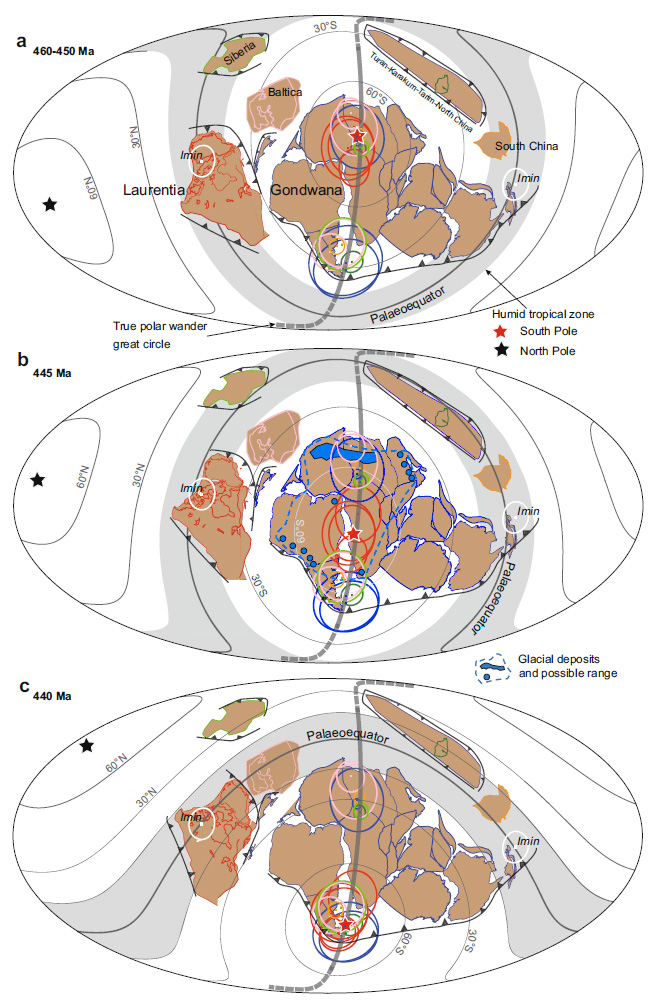
Xianqing Jing and colleagues report a wholesale 50° rotation of the lithosphere between 450 and 440 Ma that would have involved speeds of about 55 cm per year. It involved the Gondwana supercontinent and other continental masses still isolated from it moving synchronously in the same direction, as shown in the figure. From 460 to 450 Ma the geographic South Pole lay at the centre of the present Sahara. At 445 Ma its position had shifted to central Gondwana during the glacial period. By 440 Gondwana had moved further northwards so that the South Pole then lay at Gondwana’s southernmost extremity.

Palaeogeographic reconstructions charting true polar wander and the synchronised movement of all continental masses between 460 and 440 Ma. Note the changes in the trajectories of lines of latitude on the Mollweide projections. The grey band either side of the palaeo-Equator marks intense chemical weathering in the humid tropics. Credit Jing et al. Fig 5.

As well as a possible key to the brief but extreme glacial episode this astonishing journey by a vast area of lithosphere may help account for the mass extinction with rapid speciation and diversification associated with the O-S boundary. While the South Pole was traversing Gondwana as the supercontinent shifted the ‘satellite’ continental masses remained in or close to the humid tropics, exposed to silicate weathering and erosion. That is a means for extracting CO2 from the atmosphere and launching global cooling, eventually to result in glaciation over a huge tract of Gondwana around 445 Ma. Gondwana then moved rapidly into more clement climatic zones and was deglaciated a few million years later. The rapid movement of the most faunally diverse continental-shelf seas through different climate zones would have condemned earlier species to extinction simultaneous adaptation to changed conditions could have encouraged the appearance of new species and ecosystems. This does not require the catastrophic mechanisms largely established for the other mass extinction events. It seems that during the stupendous, en masse slippage of the Earth’s lithosphere plate tectonic processes still continued, yet it must have had a dynamic effect throughout the underlying mantle.

Yet the fascinating story does have a weak point. What if the position of the magnetic poles shifted during O-S times from their assumed rough coincidence with the geographic poles? In other words, did the self-exciting dynamo in the liquid outer core undergo a large and lengthy wobble? How the outer core’s circulation behaves depends on its depth to the solid core, yet the inner core seems only to have begun solidifying just before the onset of the Cambrian, about 100 Ma before the O-S events. It grew rapidly during the Palaeozoic, so the thickness of the outer core was continuously increasing. Fluid dynamic suggests that the form of its circulation may also have undergone changes, thereby affecting the shape and position of the geomagnetic field: perhaps even shifting its poles away from the geographic poles …

Annual logs for 2020 and 2021 added

For ease of access to annual developments within the general topics that Earth-logs covers I have now compiled all the Earth-logs posts from 2020 and 2021 into the categories: Geohazards; Geomorphology; Human Evolution; Magmatism; Palaeobiology; Palaeoclimatology; Physical Resources; Planetary Science; Remote Sensing; Sediments and Stratigraphy, and Tectonics. You can download them by ‘hovering’ over the Annual logs pull-down in the main menu and clicking on a category, whose index page will appear. Then scroll down to the 2020 or 2021 entry and click on the link to the PDF.

I hope that readers find this option useful in showing how each general topic has developed over the 21st century so far. Of course, it is based on my personal view of what constitute important developments published in international journals

Best wishes for 2023.

Steve Drury

Environmental DNA reveals ecology in Northern Greenland from 2 Ma ago

The closest land to the North Pole is Peary Land in northern Greenland. Today, much of it is a polar desert and is bare of ice, so field geology is possible during the Arctic summer. It is one of the last parts of the northern hemisphere to have been mapped in detail. The bedrock ranges in age from the Mesoproterozoic to Upper Cretaceous, although the sequence is incomplete because of tectonic events and erosion during the Phanerozoic Eon. Its complex history has made Peary Land a draw for both structural geologists and stratigraphers. Apart from glacial tills the youngest rocks are estuarine sediments deposited in the early Pleistocene, between two glacial tills. They define one of the earliest known interglacials, roughly between 1.9 and 2.1 Ma, which lasted for an estimated 20 ka. Late Pliocene (3.4 Ma) sediments from around the Arctic Ocean have yielded rich fossil fauna and flora that suggest much warmer conditions – 10°C higher than those at present – before repeated glaciation began in the Northern Hemisphere. The sediments in Peary Land are fossiliferous, plant remains indicating a cover of coniferous trees, but animal fossils are restricted to small invertebrates: the tangible palaeontology offers slim pickings as regards assessing environmental conditions and the ecosystem.

One means of exploring faunal and floral diversity is through sampling and analysing DNA buried in sediments and soils rather than in fossils – plants shed pollen while animals spread their DNA via dung and urine. This approach has met with extraordinary success in revealing megafaunas that may have been decimated by humans newly arrived in the Americas. Even more remarkable was the ability of environmental DNA from cave sediments to reveal the former presence of individual humans who once lived in the caves and thus assess their numbers and relatedness. Such penetrating genetic ‘fingerprinting’ only became possible when new techniques to extract fragments of DNA from sediments and splice them to reconstruct genomes had been developed. But to apply them to material some two million years old would be a big ask; The oldest known DNA sequence had been recovered in 2021 from the molar of a 1.1 Ma old mammoth preserved in permafrost – a near-ideal source. A large multinational team under the supervision of Eske Willerslev (currently of Cambridge University, UK) took on the challenge, despite two million years of burial being likely to have degraded genetic material to minuscule fragments absorbed on the surface of minerals (Kjær, K.H. and 38 others 2022. A 2-million-year-old ecosystem in Greenland uncovered by environmental DNA. Nature, v 612, p. 283–291; DOI: 10.1038/s41586-022-05453-y). But it transpired that quartz grains have a good chance of ‘collecting’ bits of DNA and readily yielding them to the extraction media. The results are extraordinary.

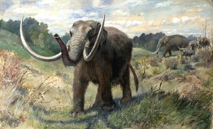
Reconstruction of an American mastodon herd by American painter of large extinct fauna Charles R. Knight

The DNA extraction turned-up signs of 70 vascular plants, including poplar, spruce and yew now typically found at much lower latitudes, alongside sedges, shrubs and birch-tree species that still grow in Greenland. The climate was substantially warmer than it is now. The fauna included elephants – probably mastodons (Mammut) but not mammoths (Mammuthus) and caribou, as well as rabbits, geese and various species of rodents. There were even signs of ants and fleas. The overall assemblage of plants has no analogue in modern vegetation, perhaps because of the absence of anthropogenic influences, such as fires, the smaller extent of glaciations, their shorter duration and less established permafrost during the early Pleistocene. The last factor could have allowed a quicker and wider spread of coniferous-deciduous woodland, found today in NE Canada. In turn this spread of vegetation would have drawn in herds of large herbivores, later mastodons being known to have been wide-ranging forest dwellers. Willerslev suggests that the study has a potential bearing on how ecosystems may respond to climate change.

Consider Homo erectus …

Championed as the earliest commonly found human species and, apart from anatomically modern humans (AMH), the most widespread through Africa and Eurasia. It also endured longer (~1.75 Ma) than any other hominin species, appearing first in East Africa around 2 Ma ago, the youngest widely accepted fossil – found in China – being around 250 ka old. The ‘erects’ arguably cooked their food and discovered the use of fire 1.7 to 2 Ma ago. The first fossils discovered in Java by Eugene Dubois are now known to be associated with the oldest-known art (430 to 540 ka) The biggest issue surrounding H. erectus has been its great diversity, succinctly indicated by a braincase capacity ranging from 550 to 1250 cm3: from slightly greater than the best endowed living apes to within the range of AMH. Even the shape of their skulls defies the constraints placed on those of other hominin species. For instance, some have sagittal crests to anchor powerful jaw muscles, whereas others do not. What they all have in common are jutting brow ridges and the absence of chins along with all more recently evolved human species, except for AMH.

This diversity is summed up in 9 subspecies having been attributed to H. erectus, the majority by Chinese palaeoanthropologists. Chinese fossils from over a dozen sites account for most of the anatomical variability, which perhaps even includes Denisovans, though their existence stems only through the DNA extracted from a few tiny bone fragments. So far none of the many ‘erect’ bones from China have been submitted to genetic analysis, so that connection remains to be tested. Several finds of diminutive humans from the Indonesian and Philippine archipelagos have been suggested to have evolved from H. erectus in isolation. All in all, the differences among the remains of H. erectus are greater than those used to separate later human species, i.e. archaic AMH, Neanderthals, Denisovans, H. antecessor etc. So it seems strange that H. erectus has not been split into several species instead of being lumped together, in the manner of the recently proposed Homo bodoensis. Another fossil cranium has turned up in central China’s Hubei province, to great excitement even though it has not yet been fully excavated (Lewis, D. 2022. Ancient skull uncovered in China could be million-year-old Homo erectus. Nature News 29 November 2022; DOI: 10.1038/d41586-022-04142-00; see also a video). Chances are that it too will be different from other examples. It also presents a good excuse to consider H. erectus.

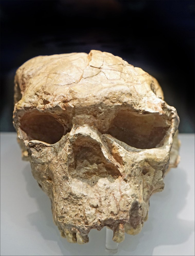
Cranium of a Chinese Homo erectus, somewhat distorted by burial, from a site close to the latest find. (Credit: Hubei Museum, Wuhan, China)

The complications began in Africa with H. ergaster, the originator of the bifacial or Acheulean multi-purpose stone tool at around 1.6 Ma (see: Flirting with hand axes; May 2009), the inventor of cooking and discoverer of the controlled use of fire. ‘Action Men’ were obviously smarter than any preceding hominin, possibly because of an increase of cooked protein and plant resources that are more easily digested than in the raw state and so more available for brain growth. The dispute over nomenclature arose from a close cranial similarity of H. ergaster to the H. erectus discovered in Java in the 19th century: H. erectus ergaster is now its widely accepted name. In 1991-5 the earliest recorded hominins outside Africa were found at Dmanisi, Georgia, in sediments dated at around 1.8 Ma (see: First out of Africa; November 2003) Among a large number of bones were five well-preserved skulls, with brain volumes less than 800 cm3 (see: An iconic early human skull; October 2013). These earliest known migrants from Africa were first thought to resemble the oldest humans (H.habilis) because of their short stature, but now are classified as H. erectus georgicus. They encapsulate the issue of anatomical variability among supposed H. erectus fossils, each being very different in appearance, one even showing ape-like features. Another had lost all teeth from the left side of the face, yet had survived long after their loss, presumably because others had cared for the individual.

The great variety of cranial forms of the Asian specimens of H. erectus may reflect a number of factors. The simplest is that continuous presence of a population there for as long as 1.5 Ma inevitably would have resulted in at least as much evolution as stemmed from the erects left behind in Africa, up to and including the emergence of AMH in North Africa about 300 ka ago. If contact with the African human population was lost after 1.8 Ma, the course of human evolution in Africa and Asia would clearly have been different. But that leaves out the possibility of several waves of migrants into Asia that carried novel physiological traits evolved in Africa to mix with those of earlier Asian populations. From about 1 Ma ago a succession of migrations from Africa populated Europe – H. antecessor, H. heidelbergensis, and Neanderthals and then AMH. So a similar succession of migrants could just as well have gone east instead of west on leaving Africa. Asia is so vast that migration may have led different groups to widely separated locations, partially cut-off by mountain ranges and deserts so that it became very difficult for them to maintain genetic contact. Geographic isolation of small groups could lead to accelerated evolution, similar to that which may have led to the tiny H. floresiensis and H. luzonensisdiscovered on Indonesian and Philippine islands.

 Another aspect of the Asian continent is its unsurpassed range of altitude, latitude and climate zones. Its ecologically diversity offers a multitude of food resources, and both climate and elevation differences pose a range of potential stresses to which humans would have had to adapt. The major climate cycles of the Pleistocene would have driven migration across latitudes within the continent, thereby mixing groups with different physical tolerances and diets to which they had adapted. Equally, westward migration was possible using the Indo-Gangetic plains and the shore of the Arabian Sea: yet more opportunities for mixing between established Asians and newly arrived African emigrants.

How did the earliest animals feed?

Among the strange early animals of the latest Precambrian, known as the Ediacaran fauna, is the slug-like Kimberella. Unlike most of its cohort, which are impressions in sediment or trace fossils,  Kimberella is a body fossil in which can be seen signs of a front and back, i.e. mouth and anus (See also: A lowly worm from the Ediacaran?). In that respect they are the same as us: bilaterians both. Indeed, Kimberella may be one of the oldest of our broad kind that we will ever be able to see. Rare examples have fans of grooves radiating from their ‘front’. It may have grated its food, a bit like a slug does, but drew it in to its mouth. Some enthusiasts have likened the little beasty to a JCB digger, able to rotate and rake stuff into its mouth. In that case, Kimberella would have moved ‘backwards’ while feeding. If it can be likened to any modern animals, it may be a simple mollusc.

A Kimberella fossil, about 10 centimetres long, and a speculative reconstruction showing its feeding apparatus.

Other Ediacaran animals show no such mouth-gut-anus symmetry. Some have tops and bases, but most show no symmetry at all, being flaccid bag-like creatures. Palaeontologists provisionally suggest that they are primitive sponges, ctenophores, placozoans and cnidarians. Such animals excrete through pores on their surfaces and draw food in either through a simple mouth or their skins. The early bilaterians probably ‘grazed’ on bacterial or algal mats, but until now that has been conjectural. Ilya Bobrovskiy of the Australian National University and colleagues from Russia and Australia have managed to extract and analyse biomarker chemicals contained in well-preserved specimens of three Ediacaran animals from strata on the White Sea coast of Russia (Bobrovskiy, I. et al. 2022. Guts, gut contents, and feeding strategies of Ediacaran animals. Current Biology, v. 32,   ; DOI: 10.1016/j.cub.2022.10.051). Biomarkers are molecules, such as fatty acids, phospholipids, triglycerides, hopanes and steranes, that definitively indicate metabolic processes of once living organisms, sometimes referred to as ‘molecular fossils’. Their varying proportions relative to one another are key to recognising the presence of different groups of organisms.

Specifically, hopane molecules are the best indicators of the former metabolism of bacteria whereas steranes (based on linked chains of carbon atoms bonded in rings) are typical products of degradation of sterols in eukaryotes. One sterane group involving 27 carbon atoms (C27 steranes) are typically formed when and animal dies and decays.   C28 and C29 steranes likely form when algae decay, as when they are digested in the gut of a herbivore. Specimens of one of the Ediacaran animals analysed by the team – Dickinsonia – contained far more C27 steranes than C28 and C29, a sign of biomarkers associated with its decay. It probably absorbed food, weirdly, through its skin. Kimberella and a worm-like animal – Calyptrina – had sterane proportions which suggested that they digested algae or bacteria in a gut, as befits bilaterians. Simple as they may appear, these are among the earliest ancestors of modern animals, including us: of course!

See also: Lu, D. 2022. The real paleo diet: researchers find traces of world’s oldest meal in 550m-year-old fossil. The Guardian, 22 November 2022.;  World’s oldest meal helps unravel mystery of our earliest animal ancestors. scimex, 23 November 2022

Early land plants and oceanic extinctions

In September 2022 Earth-logs highlighted how greening of the continents affected the composition of the continental crust. It now seems that was not the only profound change that the first land plants wrought on the Earth system. Beginning in the Silurian, the spread of vegetation swept across the continents during the Devonian Period. From a height of less than 30 cm among the earliest species by the Late Devonian the stature of plants went through a large increase with extensive forests of primitive tree-sized conifers, cycads, horsetails and sporiferous lycopods up to 10 m tall. Their rapid evolution and spread was not hampered by any herbivores. It was during the Devonian that tetrapod amphibians emerged from the seas, probably feeding on burgeoning terrestrial invertebrates. The Late Devonian was marked by five distinct episodes of extinction, two of which comprise the Devonian mass extinction: one of the ‘Big Five’. This affected both marine and terrestrial organisms. Neither flood volcanism nor extraterrestrial impact can be linked to the extinction episodes. Rather they marked a long drawn-out period of repeated environmental stress.

Phytoplankton bloom off the east coast of Scotland ‘fertilised’ by effluents carried by the Tay and Forth estuaries.

One possibility is that a side effect of the greening of the land was the release of massive amounts of nutrients to the seas that would have resulted in large-scale blooms of phytoplankton whose death and decay depleted oxygen levels in the water column. That is a process seen today where large amounts of commercial fertilisers end up in water bodies to result in their eutrophication. Matthew Smart and others from Indiana University-Purdue University, USA and the University of Southampton, UK, geochemically analysed Devonian lake deposits from Greenland and Scotland to test this hypothesis (Smart, M.S. et al. 2022. Enhanced terrestrial nutrient release during the Devonian emergence and expansion of forests: Evidence from lacustrine phosphorus and geochemical records. Geological Society of America Bulletin, v. 134, early release article;  DOI: 10.1130/B36384.1).

Smart et al. show that in the Middle and Late Devonian the lacustrine strata show cycles in their abundance of phosphorus (P an important plant nutrient) that parallel evidence for wet and dry cycles in the lacustrine basins. The cycles show that the same phosphorus abundance patterns occurred at roughly the same times at five separate sites. This may suggest a climatic control forced by changes in Earth’s orbital behaviour, similar to the Milankovich Effect on the Pleistocene climate and at other times in Phanerozoic history. The wet and dry intervals show up in the changing ratio between strontium and copper abundances (Sr/Cu): high values signify wet conditions, low suggesting dry. The wet periods show high ratios of rubidium to strontium (Rb/Sr) that suggest enhanced weathering, while dry periods show the reverse – decreased weathering.

When conditions were dry and weathering low, P built up in the lake sediments, whereas during wet conditions P decreases; i.e. it was exported from the lakes, presumably to the oceans. The authors interpret the changes in relation to the fate of plants under the different conditions. Dry periods would result in widespread death of plants and their rotting, which would release their P content to the shallowing, more stagnant lakes. When conditions were wetter root growth would have increased weathering and more rainfall would flush P from the now deeper and more active lake basins. The ultimate repository of the sediments and freshwater, the oceans, would therefore be subject to boom and bust (wet and dry) as regards nutrition and phytoplankton blooms. Dead phytoplankton, in turn, would use up dissolved oxygen during their decay. That would lead to oceanic anoxia, which also occurred in pulses during the Devonian, that may have contributed to animal extinction.

See also: Linking mass extinctions to the expansion and radiation of land plants, EurekaAlert 10 November 2022; Mass Extinctions May Have Been Driven by the Evolution of Tree Roots, SciTechDaily, 14 November 2022.

Family links among the Neanderthals of Siberia

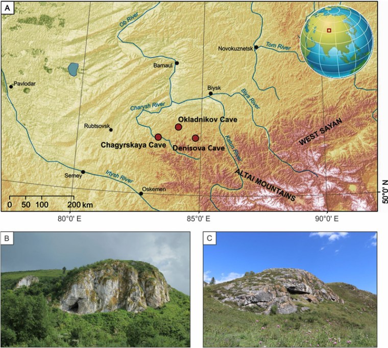
Caves used by the Neanderthals of southern Siberia: A – location map; B – Chagyrskaya Cave; C – Okladnikov Cave. (Credit: adapted from Skov et al.; Extended Data Fig. 1)

The early focus on Neanderthals was on remains found in Western Europe from the 19th century onwards. That has shifted in recent years to southern Siberia in the foothills of the Altai mountains, despite the fossils’ fragmentary nature: a few teeth and bits of mandible. The Denisova Cave became famous not just because it contained the easternmost evidence of Neanderthal occupation but through the genetic analysis of a tiny finger-tip bone. It proved not to be from a Neanderthal but a distinctly different hominin species, dubbed Denisovan (see: Other rich hominin pickings; May 2010). What Denisovans looked like remains unknown but genetic traces of them are rife among living humans of the western Pacific islands and Australia, whose ancestors interbred with Denisovans, presumably in East Asia. Modern people indigenous to Europe and the Middle East have Neanderthal genes in their genomes. Other bone fragments from Denisova Cave also yielded Neanderthal genomes, and the cave sediments yielded traces of both groups (see: Detecting the presence of hominins in ancient soil samples; April 2017). Then in 2018 DNA extracted from a limb bone from the cave clearly showed that it was from a female teenager who had had a Neanderthal mother and a Denisovan father (see: Neanderthal Mum meets Denisovan Dad; August 2018). These astonishing and unexpected finds spurred further excavations and genetic analysis in other caves within 100 km of Denisova Cave. This was largely led by current and former co-workers of Svanti Pääbo, of the Max Planck Institute for Evolutionary Anthropology, Leipzig, Germany: Pääbo was awarded the 2022 Nobel Prize in Physiology or Medicine for his coordination of research and discoveries concerning ancient human genomes. Their enormous field and laboratory efforts have paid astonishingly valuable dividends (Skov, L. and 34 others 2022. Genetic insights into the social organization of Neanderthals. Nature v. 610, p. 519–525; DOI: 10.1038/s41586-022-05283-y).

To the previously analysed 18 Neanderthal genomes from 14 archaeological sites across Eurasia (including Denisova Cave) Skov et al. have added 13 more from just two sites in Siberia (the Chagyrskaya and Okladnikov caves). Each site overlooks valleys along which game still migrates, so they may have been seasonal hunting camps rather than permanent dwellings: they are littered with bison and horse bones. Tools in the two 59-51 ka old human occupation levels are different from those at the older (130 to 91 Ka) Denisova Cave about 100 km to the east. As at the much older site, human fossils include several teeth and fragments of bones from jaws, hands, limbs and vertebrae. The detailed genomes recovered from 17 finds shows them to be from 14 individuals (12 from Chagyrskaya, 2 from Okladnikov).

Chagyrskaya yielded evidence for 5 females (3 adults and 2 children) and 7 males (3 children and 4 adults). One female estimated to have lost a premolar tooth when a teenager was the daughter of a Chagyrskaya adult male. He, in turn, was brother or father to another male, so the girl seems to have had an uncle as well. Another male and female proved to be second-degree relations (includes uncles, aunts, nephews, nieces, grandparents, grandchildren, half-siblings, and double cousins). The two people from Okladnikov were an adult female and an unrelated male child. The boy was not related to the Chagyrskaya group, but the woman was, her former presence at that cave lingering in its cave-sediment DNA. None of the newly discovered individuals were closely related to six of the seven much older Denisova Cave Neanderthals, but the Okladnikov boy had similar mtDNA to one individual from Denisova.

Further information about the Chagyrskaya group came from comparison of DNA in Y-chromosomes and mitochondria. The father of the teenage girl had two types of mtDNA – the unusual characteristic of heteroplasmy – that he shared with two other males. This suggests that three of the males shared the same maternal lineage – not necessarily a mother – and also indicates that they lived at roughly the same time. The mtDNA recovered from all Chagyrskaya individuals was much more varied than was their Y-chromosome DNA (passed only down male lineage). One way of explaining that would be females from different Neanderthal communities having migrated into the Chagyrskaya group and mated with its males, who largely remained in the group: a ‘tradition’ known as patrilocality, which is practised in traditional Hindu communities, for instance.

So, what has emerged is clear evidence for a closely related community of Neanderthals at Chagyrskaya, although it cannot be shown that all were present there at the same time, apart from the five who show first- or second-degree relatedness or mitochondrial heteroplasmy. Those represented only by individual teeth didn’t necessarily die there: adult teeth can be lost through trauma and deciduous teeth fall out naturally. There was also some individual physical connection between the two caves: The Okladnikov woman’s DNA being in the sediment at Chagyrskaya. Looking for DNA similarities more widely, it appears that all individuals at Chagyrskaya may have had some ancestral connection with Croatian Neanderthals, as did the previously mentioned mother of the Denisovan-Neanderthal hybrid girl. Four of the Chagyrskaya individuals can also be linked genetically to Neanderthals from Spain, more so than to much closer individuals found in the Caucasus Mountains. So, by around 59-51 ka the results of a wave of eastward migration of Neanderthals had reached southern Siberia. Yet the apparent matrilineal relatedness of the Okladnikov boy to the much older Neanderthals of Denisova Cave suggests that the earlier group continued to exist.

The new results are just as fascinating as the 2021 discovery that ancient DNA from Neolithic tomb burials in the Cotswolds of SW England suggests that the individual skeletons represent five continuous generations of one extended family. The difference is that they were farmers tied to the locality, whereas the Siberian Neanderthals were probably hunter gatherers with a very wide geographic range.  Laurits Skov and his colleagues have analysed less than one-quarter of the Neanderthal remains already discovered in Chagyrskaya and Okladnikov caves and only a third of the cave deposits have been excavated. Extracting and analysing ancient DNA is now far quicker, more detailed and cheaper than it was in 2010 when news of the first Neanderthal genome broke. So more Neanderthal surprises may yet come from Siberia. Progress on the genetics of their anatomically-modern contemporaries in NE Asia has not been so swift.

See also:  Callaway, E. 2022. First known Neanderthal family discovered in Siberian cave.  Nature online 19 October 2022.

Origin of animals at a time of chaotic oxygen levels

Every organism that you can easily see is a eukaryote, the vast majority of which depend on the availability of oxygen molecules. The range of genetic variation in a wide variety of eukaryotes suggests, using a molecular ‘clock’, that the first of them arose between 2000 to 1000 Ma ago. It possibly originated as a symbiotic assemblage of earlier prokaryote cells ‘bagged-up’ within a single cell wall: Lynn Margulis’s hypothesis of endosymbiosis. It had to have happened after the Great Oxygenation Event (GOE 2.4 to 2.2 Ga), before which free oxygen was present in the seas and atmosphere only at vanishingly small concentrations. Various single-celled fossil possibilities have been suggested to be the oldest members of the Eukarya but are not especially prepossessing, except for one bizarre assemblage in Gabon. The first inescapable sign that eukaryotes were around is the appearance of distinctive organic biomarkers in sediments about 720 Ma old. The Neoproterozoic is famous for its Snowball Earth episodes and the associated multiplicity of large though primitive animals during the Ediacaran Period (see: The rise of the eukaryotes; December 2017).

The records of carbon- and sulfur isotopes in Neo- and Mesoproterozoic sedimentary rocks are more or less flat lines after a mighty hiccup in the carbon and sulfur cycles that followed the GOE and the earliest recorded major glaciation of the Earth. The time between 2.0 and 1.0 Ga has been dubbed ‘the Boring Billion’. At about 900 Ma, both records run riot. Sulfur isotopes in sediments reveal the variations of sulfides and sulfates on the seafloor, which signify reducing and oxidising conditions respectively.  The δ13C record charts the burial of organic carbon and its release from marine sediments related to reducing and oxidising conditions in deep water. There were four major ‘excursions’ of δ13C during the Neoproterozoic, which became increasingly extreme. From constant anoxic, reducing conditions throughout the Boring Billion the Late Neoproterozoic ocean-floor experienced repeated cycles of low and high oxygenation reflected in sulfide and sulfate precipitation and by fluctuations in trace elements whose precipitation depends on redox conditions. By the end of the Cambrian, when marine animals were burgeoning, deep-water oxic-anoxic cycles had been smoothed out, though throughout the Phanerozoic eon anoxic events crop up from time to time.

Atmospheric levels of free oxygen relative to that today (scale is logarithmic) computed using combined carbon- and sulfur isotope records from marine sediments since 1500 Ma ago. The black line is the mean of 5,000 model runs, the grey area represents ±1 standard deviations. The pale blue area represents previous ‘guesstimates’. Vertical yellow bars are the three Snowball Earth events of the Late Neoproterozoic (Sturtian, Marinoan and Gaskiers). (Credit: Krause et al., Fig 1a)

The Late Neoproterozoic redox cycles suggest that oxygen levels in the oceans may have fluctuated too. But there are few reliable proxies for free oxygen. Until recently, individual proxies could only suggest broad, stepwise changes in the availability of oxygen: around 0.1% of modern abundance after the GOE until about 800 Ma; a steady rise to about 10% during the Late Neoproterozoic; a sharp rise to an average of roughly 80% at during the Silurian attributed to increased photosynthesis by land plants. But over the last few decades geochemists have devised a new approach based on variations on carbon and sulfur isotope data from which powerful software modelling can make plausible inferences about varying oxygen levels. Results from the latest version have just been published (Krause, A.J. et al. 2022. Extreme variability in atmospheric oxygen levels in the late Precambrian. Science Advances, v. 8, article 8191; DOI: 10.1126/sciadv.abm8191).

Alexander Krause of Leeds University, UK, and colleagues from University College London, the University of Exeter, UK and the Univerisité Claude Bernard, Lyon, France show that atmospheric oxygen oscillated between ~1 and 50 % of modern levels during the critical 740 to 540 Ma period for the origin and initial diversification of animals. Each major glaciation was associated with a rapid decline, whereas oxygen levels rebounded during the largely ice-free episodes. By the end of the Cambrian Period (485 Ma), by which time the majority of animal phyla had emerged, there appear to have been six such extreme cycles.

Entirely dependent on oxygen for their metabolism, the early animals faced periodic life-threatening stresses. In terms of oxygen availability the fluctuations are almost two orders of magnitude greater than those that animal life faced through most of the Phanerozoic. Able to thrive and diversify during the peaks, most animals of those times faced annihilation as O2 levels plummeted. These would have been periods when natural selection was at its most ruthless in the history of metazoan life on Earth. Its survival repeatedly faced termination, later mass extinctions being only partial threats. Each of those Phanerozoic events was followed by massive diversification and re-occupation of abandoned and new ecological niches. So too those Neoproterozoic organism that survived each massive environmental threat may have undergone adaptive radiation involving extreme changes in their form and function. The Ediacaran fauna was one that teemed on the sea floor, but with oxygen able to seep into the subsurface other faunas may have been evolving there exploiting dead organic matter. The only signs of that wholly new ecosystem are the burrows that first appear in the earliest Cambrian rocks. Evolution there would have ben rife but only expressed by those phyla that left it during the Cambrian Explosion.

There is a clear, empirical link between redox shifts and very large-scale glacial and deglaciation events. Seeking a cause for the dramatic cycles of climate, oxygen and life is not easy. The main drivers of the greenhouse effect COand methane had to have been involved, i.e. the global carbon cycle. But what triggered the instability after the ‘Boring Billion’? The modelled oxygen record first shows a sudden rise to above 10% of modern levels at about 900 Ma, with a short-lived tenfold decline at 800 Ma. Could the onset have had something to do with a hidden major development in the biosphere: extinction of prokaryote methane generators; explosion of reef-building and oxygen-generating stromatolites? How about a tectonic driver, such as the break-up of the Rodinia supercontinent? Then there are large extraterrestrial events … Maybe the details provided by Krause et al. will spur others to imaginative solutions. See also: How fluctuating oxygen levels may have accelerated animal evolution. Science Daily, 14 October 2022

Seven thousand years of cultural sharing in Europe between Neanderthals and modern humans

Two years ago material excavated from the Bacho Kiro cave in Bulgaria revealed that anatomically modern humans (AMH) had lived there between 44 and 47 ka ago: the earliest known migrants into Europe. Bacho Kiro contains evidence of occupancy by both Neanderthals and AMH. This discovery expanded the time over which Europe was co-occupied by ourselves and Neanderthals. The latter probably faded from the scene as an anatomically distinct group around 41 to 39 ka, although some evidence suggests that they lingered in Spain until ~37 ka and perhaps as late as 34 to 31 ka in the northern Ural mountains at the modern boundary of Europe and Asia. For most of Europe both groups were therefore capable of meeting over a period of seven to eight thousand years.

Aside from interbreeding, which they certainly did, palaeoanthropologists have long pondered on a range of tools that define an early Upper Palaeolithic culture known as the Châtelperronian, which also spans the same lengthy episode. But there have been sharp disagreements about whether it was a shared culture and, if so, which group inspired it. Evidence from the Grotte du Renne in eastern France suggests that the Neanderthals did abandon their earlier Mousterian culture to use the Châtelperronian approach early in the period of dual occupancy of Europe.

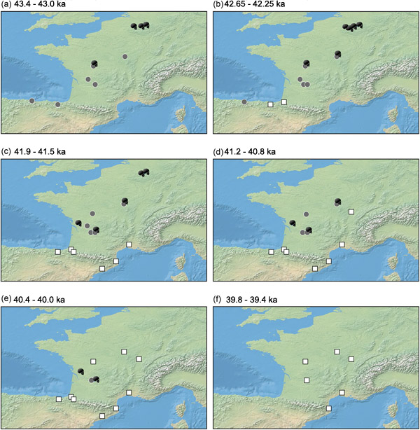
Dated appearances in France and NE Spain of Neanderthal fossils (black skulls), Châtelperronian artefacts (grey circles) and proto-Aurignacian artefacts (white squares) in different time ‘slots’ between 43.4 and 39.4 ka. (Credit: Djakovic et al., Fig. 3)

Igor Djakovic of Leiden University in the Netherlands , Alastair Key of Cambridge University, UK, and Marie Soressi, also of Leiden University have undertaken a statistical analysis of the geochronological and stratigraphic context of artefacts at Neanderthal and AMH sites in France and NW Spain during the co-occupancy period (Djakovic, I., Key, A. & Soressi, M. 2022. Optimal linear estimation models predict 1400–2900 years of overlap between Homo sapiens and Neandertals prior to their disappearance from France and northern Spain. Scientific Reports, v. 12, article  15000; DOI: 10.1038/s41598-022-19162-z). Their study is partly an attempt to shed light on the ‘authorship’ of the novel technology. The results suggest that the Châtelperronian (Ch) started around 45 ka and had disappeared by ~40.5 ka, along with the Neanderthals themselves. Early AMH artefacts are known as proto-Aurignacian (PA) and bear some resemblance to those of Châtelperronian provenance. The issue revolves around 3 conceivable scenarios: 1. the earliest AMH migrants brought the PA culture with them that Neanderthals attempted to copy, leading to their Ch tools; 2. Neanderthals independently invented the Ch methodology, which AMH adopted to produce PA artefacts; 3. both cultures arose independently.

Djakovic and colleagues have found that the data suggest that the proto-Aurignacian first appeared in the area at around 42.5 ka. Maps of dated human remains and artefacts for six 400-year time ranges from 43.4 to 39.4 ka show only Neanderthal remains and Châtelperronian artefacts from the earliest range (a in the figure). Two sites with proto-Aurignacian artefacts appears in NW Spain during the next ‘slot’ (b) then grow in numbers (c to e) relative to those of Châtelperronian provenance, which are not present after 40 ka (f) and neither are Neanderthal remains. These data suggest that local Neanderthals may have made the technological breakthrough before the appearance of the AMH proto-Aurignacian culture, which supports scenario 2 but not 1. They also suggest that the sudden appearance of Ch in France and Spain and the abandonment of earlier Neanderthal artefacts known as Mousterian could indicate that the Ch culture may have been introduced by Neanderthals migrating into the area, perhaps from further east where they may have been influenced by the earliest known European AMH in Bulgaria: i.e. tentative support for 1 or 2.

However, well documented as Djakovic et al.’s study is, it considers only 17 sites across only a fraction of Europe and a mere 28 individual artefacts each from Neanderthal and AMH associations (56 altogether). More sites and data are bound to emerge. But the study definitely opens exciting new possibilities for cultural ‘cross fertilisation’ as well as the proven physical exchange of genetic material: the two seem very likely to go hand-in-hand. Seven thousand years (~350 generations) of mutual dependence on the resources of southern Europe surely signifies too that the initially distinct groups did not engage in perpetual conflict or ecological competition, as with small numbers of both one or the other would have been extinguished within a few generations.

 See also: Devlin, H. 2022. Neanderthals and modern humans may have copied each other’s tools. The Guardian, 13 October 2022; Davis, N. 2020. Humans and Neanderthals ‘co-existed in Europe for far longer than thought’. The Guardian, 11 May 2020.

Amber, palaeontologists and a military dictatorship

Most people are familiar with the term ‘blood diamonds’, meaning diamonds clandestinely exported from areas infested by the lethal activities of military and paramilitary forces. Indeed such conflicts are often fuelled by the large profits to be made from trading diamonds.  One such source was in Sierra Leone during the civil war of 1991-2002. Others include Liberia, Côte d’ Ivoire, Angola and the Democratic Republic of Congo. Like illicit money, gemstones can be ‘laundered’ and find their way into conventional trade. To some extent the blood diamond trade has been slowed down by a programme of certification of packaged uncut diamond ‘rough’ by bona fide producers, and banning the sale of uncertified rough. The Kimberley Programme has been criticised because certificates can be issued in corrupt ways, so that blood diamonds probably still make their way to the international diamond markets: certification may hold no fears for those who force people to ine at gun point. However, because diamonds often show geochemical signatures and minute inclusions of other minerals that are unique to individual pipe-like intrusions of kimberlite that carry deep-mantle material to the surface. So, it is technically possible – but costly – to check for suspect rough. Such controls do not apply to other gemstones. A major source of very-high value gems is Myanmar (formerly Burma), whose widely condemned military dictatorship may be engaged in their unethical trade, including smuggling to neighbouring Thailand and China to avoid scrutiny.

Foot of bird chick preserved in Cretaceous amber from Kachin, Myanmar. Credit: Pinterest, Xing Lida, China University of Geosciences)

Myanmar is well endowed with sedimentary deposits that contain amber, the solidified resin from a variety of now extinct trees. Oddly, completely clear amber has low intrinsic value: it is semi-precious, albeit attractive. But it often contains inclusions of vegetation fragments, insects, feathers and small vertebrates, of interest to palaeontologists. Myanmar amber is especially interesting as it is dated to the Middle Cretaceous (~130 Ma), older than that found around the Baltic Sea (Eocene ~44 Ma), which was the main source for European jewellery since the 12th century, and that from Canada (Upper Cretaceous ~80 Ma). Myanmar amber has been used decoratively and medicinally in China since the 3rd century CE, and in Europe since prehistoric times. It is attractive but quite common, so historically amber never commanded high prices but was widely used as a trade item. Since the publicity attending the supposed extraction of dinosaur DNA from the bodies of reptile parasites to resurrect dinosaurs in Steven Spielberg’s 1993 film Jurassic Park, public and scientific interest in amber has boomed. It is primarily the exquisite preservation of encased organisms that piques the interest of palaeontologists. Papers that rely on the Myanmar amber have grown in number over the last ten years, despite the country being infamous for military repression of tribal and religious groups in its rural areas.

One of the most conflict-riven areas is the northern state of Kachin where the most interesting amber to palaeontologists is collected by the Kachin people of the Hukawng Valley. Government forces have been in conflict with the Kachin Independence Army since the 1960s, most particularly for control of the amber industry. A recent paper has focussed on the ethical issue of publications based on fossil-bearing amber from the area (Dunne, E.M. et al. 2022. Ethics, law, and politics in palaeontological research: The case of Myanmar amber. Communications Biology, v. 5, article no. 1023; DOI: 10.1038/s42003-022-03847-2).

In 2010 the military began forcibly to take over mines in Kachin.  Between 2014 and 2021 the annual number of publication underwent a tenfold growth from between 10 to 15 to over 150, despite the fact that in 2015 the government in Yangon prohibited removal of fossils from the country. But the export laws exempt gemstones, so the growing demand for fossiliferous amber is clearly reflected in its supply to foreign scientists.  Rare specimens that include vertebrate remains command prices up to US$100,000. The Myanmar amber trade is now estimated at around US$ 1 billion per annum. The Myanmar military took over all the mines in 2017, and is clearly the main supplier to palaeontologists.

In the seven-year period, only 3 papers out of 872 included contributors from Myanmar, which also suggests an element of ‘parachute science’: unsurprisingly Myanmar-based scientists also find it difficult to visit the Kachin area. Before 2014 most of the 69 publications involved scientists in the US; since then, the top spot has been occupied by Chinese scientists who have amassed 417. It seems clear that there is a web of contacts linking together the source of Myanmar amber, its market and science. In 2020 the Society of Vertebrate Paleontology called for a moratorium on publishing data from Kachin sources. But since then there is little sign that palaeontologists have taken any notice.

See also: Ortega, R.P. 2022. Violent conflict in Myanmar linked to boom in fossil amber research, study claims. Science v. 378, p.10-11; DOI: 10.1126/science.adf0973 (This commentary includes opinion that seeks to mitigate the views of Emma Dunne and colleagues)

Milankovich precession and the Palaeocene-Eocene Thermal Maximum

About 56 Ma ago there occurred some of the most dramatic biological changes since the mass extinction at the Cretaceous-Palaeogene boundary. They included rapid expansion and diversification of mammals and land plants, and a plunge in the number of deep-water foraminifera. Global cooling from the Cretaceous hothouse was rudely reversed by sudden global warming of about 5 to 10°C. Some climatologists have ascribed bugbear status to the Palaeocene-Eocene Thermal Maximum (PETM) as a possible scenario for future anthropogenic global warming. The widely accepted cause is a massive blurt into the Palaeocene atmosphere of greenhouse gases, but what caused it is enthusiastically debated. The climate shift is associated with a sudden decrease in the proportion of 13C in marine sediments: a negative spike in δ13C. Because photosynthesis favours the lighter 12C, organic matter has a low δ13C, so a great deal of buried organic carbon may have escaped from the ocean floor, most likely in the form of methane gas. However, massive burning of living terrestrial biomass would produce the same carbon-isotope signal, but absence of evidence for mass conflagration supports methane release. Methane is temporarily held in marine sediments in the form of gas hydrate (clathrate), an ice-like solid that forms at low temperatures on the deep seafloor. Warming of deep sea water or a decrease in pressure, if sea level falls, destabilise clathrates thereby releasing methane gas: the ‘clathrate gun hypothesis’. The main issue is what mechanism may have pulled the trigger for a monstrous methane release.

Massive leak of natural gas – mainly methane – off Sweden in the Baltic Sea, from the probably sabotaged Nord Stream pipeline. (Source: Swedish coastguard agency)

Many have favoured a major igneous event. Between 55.0 and 55.8 Ma basaltic magmatism– continuing today in Iceland – formed the North Atlantic Igneous Province. It involved large-scale intrusion of sills as well as outpourings of flood basalts and coincided with the initial rifting of Greenland from northern Europe (see: Smoking gun for end-Palaeocene warming: an igneous connection; July/August 2004). The occurrence of impact ejecta in end-Palaeocene sediments off the east coast of the US has spawned an extraterrestrial hypothesis for the warming, which could account for the negative spike in δ13C as the product of a burning terrestrial biosphere (see: Impact linked to the Palaeocene-Eocene boundary event; October 2016). Less headline-grabbing is the possibility that the event was part and parcel of the Milankovich effect: an inevitability in the complex interplay between the three astronomical components that affect Earth’s orbital and rotational behaviour: eccentricity, axial tilt and precession. A group of geoscientists from China and the US, led by Mingsong Li of Peking University, have investigated in minute detail the ups and downs of δ13C around 56 Ma in drill cores recovered from a sequence of Palaeocene and Eocene continental-shelf sediments in Maryland, USA (Li, M., Bralower, T.J. et al. 2022. Astrochronology of the Paleocene-Eocene Thermal Maximum on the Atlantic Coastal Plain. Nature Communications, v. 13, Article 5618; DOI: 10.1038/s41467-022-33390-x).

The study involved sampling sediment for carbon- and oxygen-isotope analysis at depth intervals between 3 and 10 cm over a 35 m section through the lower Eocene and uppermost Palaeocene. Calcium abundances in the core were logged at a resolution of 5 mm using an X-ray fluorescence instrument. The results link to variations in CaCO3 in the sediments across the PETM event. Another dataset involves semi-continuous measurements of magnetic susceptibility (MS) along the core. These measurements are able to indicate variations in delivery to the ocean of dissolved calcium and detrital magnetic minerals as climate and continental weathering vary through time. They are widely known to be good recorders of Milankovich cycles. After processing, the Ca and MS data sets show cyclical fluctuations relative to depth within the cores. ‘Tuning’ their frequencies to the familiar time series of Milankovich astronomical climate forcing reveals a close match to what would be expected if the climate fluctuations were paced by the 26 ka axial precession signal. My post of 17 June 2022 about the influence of precession over ‘iceberg armadas’ during the Pleistocene might be useful to re-read in this context. This correlation enabled the researchers to convert depth in the cores to time, so that the timing of fluctuations in carbon- and oxygen-isotope data that the PETM had created could be considered against various hypotheses for its cause. The ‘excursions’ of both began at the same time and reached the maxima of their changes from Palaeocene values over about 6,000 years. The authors consider that is far too long to countenance the release of methane as a result of asteroidal impact, or by massive burning of terrestrial vegetation. The other option that the beginning of the North Atlantic Igneous Province had been the trigger may also be ruled out on two grounds: the magmatism began earlier, and it continued for far longer. The onset of the PETM coincides with an extreme in precession-related climatic forcing. So Li et al. consider that a quirk in the Milankovich Effect could have played a role in triggering massive methane release. This might also explain features of the global calcium record in seafloor sediments as results of a brief period of ocean acidification during the PETM. Such an event would play havoc with carbonate-secreting organisms, such as foraminifera, by lowering the dissolved carbonate ion content on which they depend for their shells: hence their suffering considerable extinction. Of course, the other elements of astronomical forcing – eccentricity and axial tilt – would also have been operating on global climate at the time.  The long-term 100 and 405 ka eccentricity cycles may have played a role in amplifying warming, which may have resulted in increased burial of organic carbon and thus the amount of methane buried beneath the seabed.

British government fracking fan fracked

In November 2019 the Conservative government of Boris Johnson declared a moratorium on development of shale gas by hydraulic fracturing (‘fracking’) in England. This followed determined public protests at a number of potential fracking sites, the most intransigent being residents of Lancashire’s Fylde peninsula. They had been repeatedly disturbed since mid 2017 by low-magnitude earthquakes following drilling and hydraulic-fluid injection tests by Cuadrilla Resources near Little Plumpton village. Their views were confirmed in a scientific study by the British Geological Survey for the Oil and Gas Authority that warned of the impossibility of predicting the magnitude of future earthquakes that future fracking might trigger. The shale-gas industry of North America, largely in areas of low population and simple geology, confirmed the substantial seismic hazard of this technology by regular occurrences of earthquakes up to destructive magnitudes greater than 5.0. The Little Plumpton site was abandoned and sealed in February 2022.

Cuadrilla’s exploratory fracking site near Little Plumpton in Fylde, Lancashire. (Credit: BBC)

On 22 September 2022 the moratorium was rescinded by Jacob Rees-Mogg, Secretary of State for Business, Energy and Industrial Strategy in the new government of Liz Truss, two weeks after his appointment. This was despite the 2019 Conservative manifesto pledging not to lift the moratorium unless fracking was scientifically proven to be safe. His decision involved suggesting that the seismicity threshold for pausing fracking operations be lifted from magnitude 0.5 to 2.5, which Rees-Mogg claimed without any scientific justification to be ‘a perfectly routine natural phenomenon’.  He further asserted that opposition to fracking was based around ‘hysteria’ and public ignorance of seismological science, and that some protestors had been funded by Vladimir Putin. In reality the Secretary of State’s decision was fuelled by the Russian Federation’s reducing gas supplies to Europe following its invasion of Ukraine, the soaring world price of natural gas and an attendant financial crisis. There was also a political need to be seen to be ‘doing something’, for which he has a meagre track record in the House of Commons. Rees Mogg claimed that lifting the moratorium would bolster British energy security. That view ignored the probable lead time of around 10 years before shale gas can become an established physical resource in England. Furthermore, an August 2018 assessment of the potential of UK shale-gas, by a team of geoscientists, including one from the British Geological Survey, suggested that shale-gas potential would amount to less than 10 years supply of UK needs: contrary to Rees-Mogg’s claim that England has ‘huge reserves of shale’. Indeed it does, but the vast bulk of these shales have no commercial gas potential.

Ironically, the former founder of Cuadrilla Resources, exploration geologist Chris Cornelius, and its former public affairs director, Mark Linder, questioned the move to unleash fracking in England, despite supporting shale-gas operations where geologically and economically appropriate. Their view is largely based on Britain’s highly complex geology that poses major technical and economic challenges to hydraulic fracturing. Globally, fracking has mainly been in vast areas of simple, ‘layer-cake’ geology. A glance at large-scale geological maps of British areas claimed to host shale-gas reserves reveals the dominance of hundreds of faults, large and small, formed since the hydrocarbon-rich shales were laid down. Despite being ancient, such faults are capable of being reactivated, especially when lubricated by introduction of fluids. Exactly where they go beneath the surface is unpredictable on the scales needed for precision drilling.  Many of the problems encountered by Cuadrilla’s Fylde programme stemmed from such complexity. Over their 7 years of operation, hundreds of millions of pounds were expended without any commercial gas production. Each prospective site in Britain is similarly compartmentalised by faulting so that much the same problems would be encountered during attempts to develop them. By contrast the shales fracked profitably in the USA occur as horizontal sheets deep beneath entire states: entirely predictable for the drillers. In Britain, tens of thousands of wells would need to be drilled on a ‘compartment-by-compartment’ basis at a rate of hundreds each year to yield useful gas supplies. Fracking in England would therefore present unacceptable economic risks to potential investors. Cornelius and Linder have moved on to more achievable ventures in renewables such as geothermal heating in areas of simple British geology.

Jacob Rees-Mogg’s second-class degree in history from Oxford and his long connection with hedge-fund management seem not to be appropriate qualifications for making complex geoscientific decisions. Such a view is apparently held by several fellow Conservative MPs, one of whom suggested that Rees-Mogg should lead by example and make his North East Somerset constituency the ‘first to be fracked’, because it is underlain by potentially gas-yielding shales. The adjoining constituency, Wells, has several sites with shale-gas licences but none have been sought within North East Somerset. Interestingly, successive Conservative governments since 2015, mindful of a ‘not-in-my-backyard’ attitude in the party’s many rural constituencies, have placed a de-facto ban on development of onshore wind power.

A Lower Jurassic environmental crisis

Curiously, one of the largest environmental disruptions during the Phanerozoic Eon (i.e. since 541 Ma ago) does not stand out in the way that the ‘Big Five’ mass extinctions do. Each of them killed off between 70 and 95% of all marine species. The Jurassic was a period of biological recovery from the End-Triassic extinction 201 Ma ago. Throughout its ~50 Ma duration extinction rates were below the average for the Phanerozoic, and they remained relatively low until the K-Pg mass extinction that drew the Mesozoic Era to a close at 66 Ma. Nevertheless, there were significant extinctions, such as the demise of several lineages of herbivorous dinosaurs towards the end of the Early Jurassic followed by the rise of the familiar, long-necked variety of eusauropods. Marine organisms that secreted hard parts made of calcium carbonate also experienced a collapse then. From time to time during the Jurassic and Cretaceous Periods the oceans lost a great deal of dissolved oxygen, increasing the chances of organic carbon being buried in marine sediments. Such oceanic anoxia resulted in the widespread deposition of hydrocarbon source rocks in the form of black bituminous muds. Overall, both the Jurassic and Cretaceous experienced  greenhouse climatic conditions, with  atmospheric CO2 levels rising to almost 3000 ppm and oxygen levels significantly lower than the modern 21%. Sea levels rose by up to 200 metres, thought to be due to fast sea-floor spreading and large areas of warm, buoyant oceanic lithosphere.

A notable ocean-anoxia event took place during the Lower Jurassic, around 183 Ma ago at the start of the Toarcian Age. This stratigraphic level was penetrated by a 1.5 km borehole sunk in 2015-2016 at Mochras in North Wales, UK, on the shore of Cardigan Bay. The core provided the thickest and most complete record ever recovered for this event, and has been analysed in exquisite detail using many techniques. The most revealing data have been published by a multinational team led by scientists from Trinity College, Dublin (Ruhl, M. et al. 2022. Reduced plate motion controlled timing of Early Jurassic Karoo-Ferrar large igneous province volcanism. Science Advances, v. 8, article eabo0866; DOI: 10.1126/sciadv.abo0866).

Plate boundaries around Gondwanaland and the Karoo-Ferrar large igneous province in the Early Jurassic (small yellow dots show dated localities) . Large pink dots: positions of Tristan de Cunha and Bouvet hotspots at the time (Credit: Ruhl et al. Fig 1A)

At the start of the Toarcian (183.7 Ma) the 187Os/186Os ratio of the samples begins to rise from 0.3 to almost 0.8 to fall back to 0.3 by 180.8 Ma. Osmium isotopes are a measure of continental weathering, and this ‘excursion’ surely signifies significant global warming and increases in atmospheric humidity and acidity that broke down rocks at the continental surface. Over the same period δ13C rises, decreases to by far the lowest value in the Lower Jurassic, rises again to gradually fall back. The start of the Toarcian seems to have experienced a major release of carbon then a profound sequestration of organic carbon, presumably through burial of dead organisms in the black mudstones that signify anoxic conditions. Remarkably, the 95 m thick Toarcian black-mudstone sequence also reveals a tenfold increase in its content of the element mercury, from 20 to 200 parts per billion (ppb), peaking at the same time (~182.8 Ma) as the most negative δ13C value was reached: the acme of carbon sequestration. A coincidence of massive organic carbon burial and increased mercury in marine sediments also happened at the time of the end-Permian mass extinction, although that does not necessarily imply exactly the same mechanism.

The early Toarcian geochemical trends, however, coincide with the initiation and duration of the Karoo-Ferrar large igneous province, which formed flood basalts, igneous dyke swarms and large volcanic centres in South Africa and Antarctica. That LIP may have emitted mercury, but so too may have increased chemical weathering of the land surface. Whichever, mercury forms an organic compound (methyl mercury) in water bodies. Readily incorporated into living organisms, that could explain the close parallel between the δ13C and Hg records in the Jurassic sediment core from Wales. The Karoo-Ferrar igneous activity itself presents a bit of a conundrum, as suggested by Ruhl et al. It happened at the very time that there was a 120° change in the direction of motion of the tectonic plate carrying along Africa and, indeed, the Gondwanaland supercontinent during the Jurassic. The directional change also involved local plate movement stopping for a while. According to the authors, it wasn’t a fortuitous coincidence of two mantle plumes from the core-mantle boundary hitting the bottom of the continental lithosphere below Africa and Antarctica at this tectonic ‘U-turn’. It is more likely that the pause gave existing plumes the opportunity and time to ‘erode’ the base of the continental lithosphere and rise. Decompression melting would then have produced the voluminous magmas. The two plumes were in place for a very long time and created seamount chains as plates moved over them. Both are still volcanically active: Tristan de Cunha on the mid-Atlantic Ridge, and Bouvet Island at a triple junction between South Africa and Antarctica.

So, a venture to unravel a period of profound environmental change during the Early Jurassic, which didn’t result in mass extinction, may well have spawned a new model for massive igneous events that did. Ruhl et al. suggest that the short-lived Siberian, North Atlantic and East African Rift LIPs each seem to have coincided with short episodes of tectonic slowing-down: LIPs may result in dramatic environmental change, but at the whim of plate tectonics.

See also: https://scitechdaily.com/surprising-discovery-shows-how-slowing-of-continental-plate-movement-controlled-earths-largest-volcanic-events/

The Earth System in action: land plants affected composition of continental crust

The essence of the Earth System is that all processes upon, above and beneath the surface interact in a bewildering set of connections. Matter and energy in all their forms are continually being exchanged, deployed and moved through complex cycles: involving rocks and sediments; water in its various forms; gases in the atmosphere; magmas; moving tectonic plates and much else besides. The central and massively dominant role of plate tectonics connects surface processes with those of our planet’s interior: the lithosphere, mantle and, arguably, the core. Interactions between the Earth System’s components impose changes in the dynamics and chemical processes through which it operates. Living processes have been a part of this for at least 3.5 billion years ago, in part through their role in the carbon cycle and thus the Earth’s climatic evolution. During the Silurian Period life became a pervasive component of the continental surface, first in the form of plants, to be followed by animals during the Devonian Period. Those novel changes have remained in place since about 430 Ma ago, plants being the dominant base of continental ecosystems and food chains.

Schematic diagram showing changes in river systems and their alluvium before and after the development of land plants. (Credit: Based on Spencer et al. 2022, Fig 4)

Land plants exude a variety of chemicals from their roots that break down rock to yield nutrient elements. So they play a dominant role in the formation of soil and are an important means of rock weathering and the production of clay minerals from igneous and metamorphic minerals. Plant root systems bind near-surface sediments thus increasing their resistance to erosion by wind and water, and to mass movement under gravity. This binding and plant canopies efficiently reduce dust transport, slow water flow on slopes and decrease the sediment load of flowing water. Plants and their roots also stabilise channels systems. There is much evidence that before the Devonian most rivers comprised continually migrating braided channels in which mainly coarse sands and gravels were rapidly deposited while silts and muds in suspension were shifted to the sea. Thereafter flow became dominated by larger and fewer channels meandering across wide tracts on which fine sediment could accumulate as alluvium on flood plains when channels broke their banks. Land plants more efficiently extract CO2 from the atmosphere through photosynthesis and the new regime of floodplains could store dead plant debris in the muds and also in thick peat deposits. As a result, greenhouse warming had dwindled by the Carboniferous, encouraging global cooling and glaciation. 

Judging the wider influence of the ‘greening of the land’ on other parts of the Earth system, particularly those that depend on internal  magmatic processes, relies on detecting geochemical changes in minerals formed as direct outcomes of plate tectonics. Christopher Spencer of Queen’s University in Kingston, Canada and co-workers at the Universities of Southampton, Cambridge and Aberdeen in the UK, and the China University of Geosciences in Wuhan set out to find and assess such a geochemical signal (Spencer, C., Davies, N., Gernon, T. et al. 2022. Composition of continental crust altered by the emergence of land plants. Nature Geoscience, v. 15 online publication; DOI: 10.1038/s41561-022-00995-2). Achieving that required analyses of a common mineral formed when magmas crystallise: one that can be precisely dated, contains diverse trace elements and whose chemistry remains little changed by later geological events. Readers of Earth-logs might have guessed that would be zircon (ZrSiO). Being chemically unreactive and hard, small zircon grains resist weathering and the abrasion of transport to become common minor minerals in sediments. Thousands of detrital zircon grains teased out from sediments have been dated and analysed in the last few decades. They span almost the entirety of geological history. Spencer et al. compiled a database of over 5,000 zircon analyses from igneous rocks formed at subduction zones over the last 720 Ma, from 183 publications by a variety of laboratories.

The approach considered two measures: the varying percentages of mudrocks in continental sedimentary sequences since 600 Ma ago; aspects of the hafnium- (Hf) and oxygen-isotope proportions measured in the zircons using mass spectrometry and their changes over the same time. Before ~430 Ma the proportion of mudrocks in continental sedimentary sequences is consistently much lower than it is in post post-Silurian, suggesting a link with the rise of continental plant cover (see second paragraph). The deviation of the 176Hf/177Hf ratio in an igneous mineral from that of chondritic meteorites (the mineral’s εHf value) is a guide to the source of the magma, negative values indicating a crustal source, whereas positive values suggest a mantle origin. The relative proportions of two oxygen isotopes 18O and 16O  in zircons, expressed as δ18O, indicates the proportion of products of weathering, such as clay minerals, involved in magma production – 18O selectively moves from groundwater to clay minerals when they form, increasing their δ18O.

While the two geochemical parameters express very different geological processes, the authors noticed that before ~430 Ma the two showed low correlation between their values in zircons. Yet, surprisingly, the parameters showed a considerable and consistent increase in their correlation in younger zircons, directly paralleling the ‘step change’ in the proportions of mudstones after the Silurian. Complex as their arguments are, based on several statistical tests, Spencer et al. conclude that the geologically sudden change in zircon geochemistry ultimately stems from land plants’ stabilisation of river systems. As a result more clay minerals formed by protracted weathering, increasing the δ18O in soils when they were eroded and transported. When the resulting marine mudrocks were subducted they transferred their oxygen-isotope proportions to magmas when they were partially melted.

That bolsters the case for dramatic geological consequences of the ‘greening of the land’. But did its effect on arc magmatism fundamentally change the bulk composition of post-Silurian additions to the continental crust? To be convinced of that I would like to see if other geochemical parameters in subduction-related magmas changed after 430 Ma. Many other elements and isotopes in broadly granitic rocks have been monitored since the emergence of high-precision rock-analysing technologies around 50 years ago. There has been no mention, to my knowledge, that the late-Silurian involved a magmatic game-changer to match that which occurred in the Archaean, also revealed by hafnium and oxygen isotopes in much more ancient zircons.   

See also: https://www.sci.news/othersciences/geoscience/land-plants-continental-crust-composition-11151.htmlhttps://www.eurekalert.org/news-releases/963296

Sun, sand and sangria on the Mediterranean Costas – and tsunamis?

You can easily spot a tourist returning from a few summer weeks on the coast of the western Mediterranean, especially during 2022’s record-breaking heat wave and wildfires: sunburnt and with a smoky aroma that expensive après-sun lotion can’t mask. Judging from the seismic records, they may have felt the odd minor earthquake too, perhaps putting it down to drink, lack of sleep and an overdose of trance music. Data from the last 100 years show that southern Spain and north-west Africa have a generally uniform distribution of seismic events, mostly less than Magnitude 5. Yet there is a distinct submarine zone running NNE to SSW from Almeria to the coast of western Algeria. It crosses the Alboran Basin, and reveals significantly more events greater than M 5. Most earthquakes in the region occurred at depths less than 30 km mainly in the crust. Five geophysicists from Spain and another two from Algeria and Italy have analysed the known seismicity of the region in the light of its tectonics and lithospheric structure (Gómez de la Peña, L., et al. 2022. Evidence for a developing plate boundary in the western Mediterranean. Nature Communications, v. 13, article 4786; DOI: 10.1038/s41467-022-31895-z).

Topography of the Alboran Basin beneath the western Mediterranean. The colours grey through blue to purple indicate increasing depth of seawater. Grey circles indicate historic earthquakes, the smallest being M 3 to 4, the largest greater than M 6. Green arrows show plate motions in the area measured using GPS. Active faults are marked in red (see key for types of motion). (Credit: based on Fig 1 of Gómez de la Peña et al.)

The West Alboran Basin is underlain by thinner continental crust (orange on the inset to the map) than beneath southern Spain and western Algeria. Normal crust underpins the Southern Alboran Basin. To the east are the deeper East Alboran and Algero-Balearic Basins, the floor of the latter being true oceanic crust and that of the former created in a now extinct island arc. Running ENE to WSW across the Alboran Basin are two ridges on the sea floor. Tectonic motions determined using the Global Positioning System reveal that the African plate is moving slowly westwards at up to 1 cm yr-1, about 2 to 3 times faster than the European plate. This reflected by the dextral strike-slip along the active ~E-W Yusuf Fault (YSF). This bends southwards to roughly parallel the Alboran Ridge, and becomes a large thrust fault that shows up on ship borne seismic reflection sections. The reflection seismic survey also shows that the shallow crust beneath the Alboran Ridge is being buckled under compression above the thrust. The thrust extends to the base of the African continental crust, which is beginning to override the arc crust of the East Alboran basin. Effectively, this system of major faults seems to have become a plate boundary between Africa and Europe in the last 5 million years and has taken up about 25 km of convergence between the two plates. An estimated 16 km of this has taken place across the Alboran Ridge Thrust which has detached the overriding African crust from the mantle beneath.

The authors estimate an 8.5 to 10 km depth beneath the Alboran fault system at which the overriding crust changes from ductile to brittle deformation – the threshold for strains being taken up by earthquakes. By comparison with other areas of seismic activity, they reckon that there is a distinct chance of much larger earthquakes (up to M 8) in the geologically near future. A great earthquake in this region, where the Mediterranean narrows towards the Strait of Gibraltar, may generate a devastating tsunami. An extension of the Africa-Europe plate boundary into the Atlantic is believed to have generated a major earthquake that launched a tsunami to destroy Lisbon and batter the Atlantic coasts of Portugal, Spain and NW Africa on 1st November 1755. The situation of the active plate boundary in the Alboran Basin may well present a similar, if not worse, risk of devastation.

The earliest upright ape

Two decades ago the world of palaeoanthropologists was in turmoil with the publication of an account of a new find in Chad (see: Bonanza time for Bonzo; July 2002). A fossil cranium, dubbed Sahelanthropus tchadensis (nicknamed Toumaï­ or ‘hope of life’ in the Goran language), appeared like a cross between a chimpanzee and an australopithecine. The turmoil erupted partly because of its age: Upper Miocene, around 7 Ma old. Such an antiquity was difficult to reconcile with the then accepted ~5 Ma estimate for the evolutionary split between humans and chimpanzees, based on applying a ‘molecular clock’ approach to the difference between their mtDNA. The other point of contention was the size of Sahelanthropus’s canine teeth: far too large for australopithecines and humans, but more appropriate for a gorilla or chimp.

Cast of the reconstructed skull of Sahelanthropus tchadensis. (Credit: Didier Descouens, University of Toulouse)

In the absence of pelvic- and foot bones, or signs of the foramen magnum where the spinal cord enters the skull – crucial in distinguishing habitual bipedalism or being an obligate quadruped – encouraged the finders of a 6.1 to 5.7 Ma-old Kenyan hominin Orrorin tugenensis to insist that its skeletal remains – several teeth, fragments of a lower jaw, a thigh bone, an upper arm and of a finger and thumb but no cranial bones – were of ‘the earliest human ancestor’. In Orrorin’s favour were smaller canine teeth than those of later australopithecines. At the time of the dispute, centred mainly on absence of crucial evidence, doyen of hominin fossils Bernard Wood of George Washington University and an advocate of ‘untidy’ evolution, suggested that both early species may well have been evolutionary ‘dead ends’ (see: A considered view; October 2002). And there the ‘muddle’ has rested for 20 years.

In 2002 not only a cranium of Sahelanthropus had been unearthed. Three lower jaw bones and a collection of teeth suggested that as many as 5 individuals had been fossilised. A partial leg bone (femur) and three from forearms (ulna) cannot definitely be ascribed to Sahelanthropus but, in the absence of evidence of any other putative hominin species, they may well be. It has taken two decades for these remains to be analysed to a standard acceptable to peer review (Daver, G. et al. 2022. Postcranial evidence of late Miocene hominin bipedalism in Chad. Nature v. 608, published online; DOI: 10.1038/s41586-022-04901-z). The authors present convoluted anatomical evidence that Toumaï­’s femur, which had been gnawed by a porcupine and lacks joints at both ends, suggesting that it was indeed suited to upright walking. Yet the arm bones hint that it may have been equally comfortable in tree canopies. Yet it does look very like an ape rather than a hominin.

Much the same conclusion has been applied to Australopithecus afarensis, indeed its celebrated representative ‘Lucy’ met her end through falling out of a large tree ~3.2 Ma ago (see: Lucy: the australopithecine who fell to Earth?; September 2016). So, dual habitats may have been adopted by hominins long after they emerged. Yet Au afarensis was capable of trudging through mud as witnessed by the famous footprints at Laetoli in Tanzania. Only around 3 Ma has reasonably convincing evidence for upright walking similar to ours been discovered in Au africanus. The full package of signs from pelvis and foot for habitual bipedalism dates to 2 Ma ago in Au sediba. Even this latest known australopithecine seems to have had a gait oddly different from that of members of the genus Homo.

So, in many respects the benefits of full freeing of the hands to develop manipulation of objects, as first suggested by Freidrich Engels, may have had to await the appearance of early humans. Earlier hominins almost certainly did make tools of a kind, but the revolutionary breakthrough associated with humanity was more than 5 million years in the making.

See also: Callaway, E. 2022. Seven-million-year-old femur suggests ancient human relative walked upright. Nature (News)24 August 2022;

Handwerk, B. 2022. Seven Million Years Ago, the Oldest Known Early Human Was Already Walking. Smithsonion Magazine, 24 August 2022 (click the link ‘published today in Nature’ in 2nd paragraph to access complimentary PDF of Daver et al)

Did giant impacts trigger formation of the bulk of continental crust?

Earth is the only one of the rocky Inner Planets that has substantial continental crust, the rest being largely basaltic worlds. That explains a lot. For a start, it means that almost 30 percent of its surface area stands well above the average level of the basaltic ocean basins – more than 5 km – because of the difference in density between continental and oceanic lithosphere. Without continents and the inability of subduction to draw them back  into the mantle  Earth would remain a water-world as it is thought to have been during the Hadean and early Archaean Eons. The complex processes involved in geochemical differentiation and the repeated reworking of the continents through continual tectonic and sedimentary processes has further enriched parts of them in all manner of useful elements and chemical compounds. And, of course, the land has had a huge biosphere since the Devonian period that subsequently helped to draw down CO­2 well as evolving us.

It has been estimated that during the Archaean (4.0 to 2.5 Ga) around 75% of continental crust formed. Much of this Archaean crust is made up of sodium-rich granitoids: grey tonalite-trondhjemite-granodiorite (TTG) gneisses in the main. Their patterns of trace elements strongly suggest that their parent magmas formed by partial melting at shallow depths (25 to 50 km). Their source was probably basalts altered by hydrothermal fluids to amphibolites, unlike the post-Archaean dominance of melting associated with subducted slabs of lithosphere. Yet most of the discourse on early continents has centred on when plate tectonics began and when they became strong enough to avoid disruption into subductible ‘chunks’. Yet 10 years ago geochemists at the University of St Andrews in Scotland used hafnium and oxygen isotopes in Archaean zircons to suggest that the first continents grew very quickly in the Hadean and early Archaean at around 3.0 km3 yr-1, slowing to an average of 0.8 km3 yr-1 after 3.5 Ga. In 2017 Geochemists working on one of the oldest cratons in the Pilbara region of Western Australia developed a new, multistage model for early crust formation that did not have a subduction component. They proposed that high degrees of mantle melting first produced a mafic-ultramafic crust of komatiites, which became the source for a 3.5 Ga mafic magma with a geochemistry similar to those of modern island-arc basalts. If a crust of that composition attained a thickness greater than 25 km and was itself partially melted at its base, theoretically it could have generated TTG magma and Archaean continental crust. Three members of that team from Curtin University, Western Australia, and others have now contributed to formulating a new possibility for early continent formation (Johnson, T.E. et al. 2022.  Giant impacts and the origin and evolution of continents. Nature, v. 608, p. 330–335; DOI: 10.1038/s41586-022-04956-y).

The distinctive Archaean granite-greenstone terrain of the Pilbara craton of Western Australia. TTG granites are shown in reds in the form of domes, which are enveloped by metamorphosed sediments and mafic-ultramafic volcanics in khaki and emerald green. Other colours signify post Archaean rocks. (Credit: Warren B. Hamilton; Earth’s first two billion years. GSA, 2007)

Tim Johnson and colleagues base their views on oxygen isotopes in Archaean zircon grains from the Pilbara. The zircons’ O-isotopes fall into three kinds of cluster: low 18O that indicate a hydrothermally altered source; intermediate 18O suggesting a mantle source; high 18O signifying contamination by metasedimentary and volcanic rocks. The first two alternate in the 3.6 to 3.4 Ga period; 4 clusters with mantle connotations occupy the 3.4 to 3.0 Ga range; a cluster with supracrustal contamination follows 3.0 Ga. This record can be reconciled agreeably with the geological and broad geochemical history of the Pilbara craton. But there is another connection: the Late Heavy Bombardment (LHB) recognised on most rocky bodies in the Solar System.

Bodies with much more sluggish internal processes than the Earth have preserved much of their earliest surfaces and the damage they have suffered since the Hadean. The Moon is the best example. Its earliest rocks in the lunar Highlands record a vast number of impact craters. Their relative ages, deduced from older ones being affected by later ones, backed up by radiometric ages of materials produced by impacts, such as melt spherules and basaltic magmas that flooded the lunar maria, revealed the time span of the LHB. The maria formed between 4.2 and 3.2 billion years ago and the damage done then is shown starkly by the dark maria that make up the ‘face’ of the Man in the Moon. The lunar bombardment was at a maximum between 4.1 and 3.8 Ga but continued until 3.5 Ga, dropping off sharply from its maximum effects. Earth preserves no tangible sign of the LHB, but because it is larger and more massive than the Moon, and both have always been in much the same orbit around the Sun, it must have been subject to impacts on a far grander scale. Projectiles carry kinetic energy that enables them to do geological work when they impact: 1/2 x mass x speed2. The minimum speed of an impact is the same as the target’s escape velocity – 2.4 km s-1 for the Moon and 11.2 km s-1 for the Earth. So the energy of an object hitting the Earth would be 20 times more than if it struck the lunar surface. Taking into account the Earth’s larger cross sectional area, the amount of geological work done here by the LHB would have been as much as 300 times greater than that on Earth’s battered satellite.

The Earth’s early geological history was rarely seen in that context before the 21st century, but that is the framework plausibly adopted by Johnson and colleagues. Archaean  sediments in South Africa contain several beds of impact spherules older than 3.2 Ga, as do those of the Pilbara. The LHB also left a geochemical imprint on Earth in the form of anomalous isotope proportions of tungsten in 3.8 Ga gneisses from West Greenland (See: Tungsten and Archaean heavy bombardment and Evidence builds for major impacts in Early Archaean; respectively, July and August 2002). Johnson et al. suggest a 3-stage process for the evolution of the Pilbara craton: First a giant impact akin to the lunar Maria that formed a nucleus of mafic-ultramafic crust from shallow melting of the mantle; its chemical fractionation to produce low-magnesium basalts; and in turn their melting to form TTG magmas and thus a continental nucleus. They conclude:

‘The search for evidence of the Late Heavy Bombardment on Earth has been a long one. However, all along it seems that the evidence was right beneath our feet.’

I agree wholeheartedly, but would add that, until quite recently, many scientists who referred to extraterrestrial influences over Earth history were either pilloried or lampooned by their peers as purveyors of ‘whizz-bang’ science. So, many ‘kept their powder dry’. The weight of evidence and a reversal of wider opinion over the last couple of decades has made such hypotheses acceptable. But it has also opened the door to less plausible notions, such as an impact cause for sudden climate change and even for mythological catastrophes such as the destruction of Sodom and Gomorrah!

See also: Timmer, J. 2022. Did giant impacts start plate tectonics? arsTechnica 11 August 2022.

Late formation of the Earth’s inner core

The layered structure of the Earth was discovered using the varying arrival times of seismic waves from major earthquakes, which pass through the Earth, at seismometer stations located across the planet’s surface. Analysis of these arrival times indicates the wavepaths taken through the planet, involving reflections and refractions at boundaries of materials with distinctly different physical properties. S-waves from an earthquake do not arrive in a wide ‘shadow zone’ around its antipode. Since that kind of wave depends on shearing and cannot pass through liquid the shadow reveals the presence of an outer core made of very dense liquid iron and nickel. P-waves that travel in a manner akin to sound waves also show a shadow but it is annular in form around the antipode because of refraction at the core-mantle boundary, but they do penetrate to reach the antipode. However, their arrival times there show faster speeds than expected from an entirely liquid core, and so reveal a central mass, the inner core, which is a ball of solid iron-nickel alloy about 70% of the Moon’s size.

The Earth’s internal structure as revealed by seismic waves (Credit: Smithsonian Institute)

Movements of liquid Fe-Ni in the outer core generate Earth’s magnetic field in the manner of a self-exciting dynamo. Motion in the outer core results from convection of heat from below – probably mainly heat generated by planetary accretion – coupled with the Earth’s rotation and the Coriolis Effect.  The present style of motion is in a thick molten layer trapped between the solid mantle and the inner core. Its circulation results in a magnetic field with two distinct poles close to the geographic ones. The field is crudely similar to that of a bar magnet, with lesser deviations spread around the planet. However, it is not particularly stable, as shown by periodic flips or reversals of polarity through geological time (see: How the core controls Earth’s magnetic field reversals; April 2005).

Few geoscientists doubt that the core formed early in Earth’s history from excess iron, nickel and sulfur, plus other siderophile elements such as gold, that cannot be accommodated by the dominant silicates of the mantle. This could not have been achieved other than by iron-rich melts sinking in some way because of their density. Gradual loss of original heat of accretion and declining radiogenic heat from rare isotopes (e.g. 40K) in the melt suggests an original, totally molten core that at some time began to crystallise under stupendous pressure in its lowest parts. A fully molten core would have been turbulent and therefore able to generate a magnetic field, and Archaean rocks still retain remanent magnetisation. The form that the field took can only be modelled. At times it may have been dipolar – paleomagnetic pole positions match geological evidence for early supercontinents –  and it may have undergone reversals. When the inner core formed has long remained disputed, yet thanks to advances in palaeomagnetic analysis it may now have been resolved  (Zhou, T. and 11 others 2022. Early Cambrian renewal of the geodynamo and the origin of inner core structure. Nature Communications, v. 13, article 4161; DOI:10.1038/s41467-022-31677-7).

Tinghong Zhou of the University of Rochester, USA, and colleagues from other US, Chinese and British institutions have assiduously measured the original magnetic intensities locked in tiny iron- and iron-titanium oxide needles trapped in feldspars that dominate plutonic igneous rocks, known as anorthosites, of late Precambrian age. They found that, by about 565 Ma ago during the Ediacaran Period, the Earth’s magnetic field strength had fallen to almost a sixth of its value in the early Archaean: about 15 times less than it is today. Within a mere 30 Ma it had risen to become 5 times its lowest value , as recorded by a Cambrian anorthosite, and then rose steadily through the Phanerozoic Eon to its present strength. Modelling of the rapid rebound suggests that the inner core had begun to crystallise by about 550 Ma to reach half its present radius by the end of the Ordovician Period (~450 Ma).

That event may also have been a milestone for the continuation of biological evolution on Earth. While Mars once probably had a molten core and magnetic field, it vanished 4 billion years ago, probably when its core became solid. Early Mars had an ocean in its northern hemisphere up to about 3.8 Ga, and there is plenty of evidence for erosion by water on its higher surfaces. For liquid water to have existed there for hundreds of million years demands a thick, warm atmosphere able to initiate a greenhouse effect. With low atmospheric pressure water could have existed only as ice or water vapour. Now its atmosphere is very thin and except at its poles there is no sign of surface water, even as ice (it is possible that significant amounts of water ice remain protected beneath the surface of Mars). One hypothesis is that when Mars lost its magnetic field it also lost protection from the stream of energetic particles known as the solar wind, which can strip water vapour and carbon dioxide – and thus their ability to retain atmospheric heat – from the top of the atmosphere. Earth is currently protected from the solar wind by its strong magnetic field and magnetosphere that deflects high-speed, charged particles. During the Ediacaran Period it almost lost that protection, but was spared by the self-exciting dynamo being regenerated.

See also: How did Earth avoid a Mars-like fate? Ancient rocks hold clues. Science Daily, 25 July 2022

The dangers of rolling boulders

Field work in lonely and spectacular places is a privilege. Though it can be great, boredom sometimes sets in, which is hard for the lone geologist. Today, I guess a cell phone would help, especially in high places where the signal is good. That means of communication and entertainment only emerged in the 1980s and did not reach wild places until well into the 90s. Pre-cellnet boredom could be relieved by what remains a dark secret: lone geologists once rolled large boulders down mountains and valley sides, shouting ‘Below!’ as a warning to others. Their excuse to themselves for this unique thrill (bounding boulders reach speeds of up to 40 m s-1) was vaguely scientific: sooner or later a precarious rock would fall anyway. This week it emerged that Andrin Caviezel of the Institute for Snow and Avalanche Research in Davos, Switzerland, an Alpine geoscientist, rolls boulders for a living (Caviezel, A. 2022. The gravity of rockfalls. Where I work, Nature, v. 607, p. 838; DOI: 10.1038/d41586-022-02044-9). He finds that ‘…flinging giant objects down a mountain is still super fun’. The serious part of his job attempts to model how rockfalls actually move downslope, as an aid to risk assessment (Caviezel, A. and 23 others 2021. The relevance of rock shape over mass – implications for rockfall hazard assessments. Nature Communications, v. 12, article 5546; DOI: 10.1038/s41467-021-25794-y)

Caviezel’s team (@teamcaviezel) don’t use actual rocks but garishly painted, symmetrical blocks of reinforced concrete weighing up to 3 tonnes, which are more durable than most outcropping rock and can be re-used. A Super Puma helicopter shifts a block to the top of a slope, from which it is levered over the edge (watch video). The team deploys two types of block, one equant and resembling a giant garnet crystal, the other wheel-shaped with facets. The first represents boulders of rock types with uniform properties throughout, such as granite. The wheel type mimics boulders formed from rocks that are bedded or foliated, which are usually plate-like or spindly.

Vertical aerial photograph of a uniform, south-facing slope in the Swiss Alps used to roll concrete ‘boulders’. The red X marks the release point; the blue symbols show the points of rest of equant ‘boulders, the sizes of which are shown in the inset, the wheel-shaped ones are magenta. Coloured circles with crosses show the mean rest position of each category (the lighter the colour the smaller the set of ‘boulders’). The coloured ellipses indicate the standard deviation for each category. (Credit: Caviezel et al., Fig 2)

Unlike other gravity-driven hazards, such as avalanches and mudflows, the directions that rockfalls may follow by are impossible to predict. Rather than hugging the surface, boulders interact with it, bouncing and being deflected, and they spin rapidly. To follow each experiment’s trajectory a block contains a motion sensor, measuring speed and acceleration, and a gyroscope that shows rotation, wobbling and motion direction, while filming records jump heights – up to 11 m in the experiments. Despite the similarity of the blocks, the same release point for each roll and a uniform mountainside slope, with one cliff line, the final resting places are widely spread. That hazard zone of rockfalls is distinctly wider than that of snow avalanches; observing a boulder once it starts to move gives a potential victim little means of knowing a safe place to shelter.

The most important conclusion from the experiments is that the widest spread of tumbling ‘boulders’ is shown by the wheel-shaped ones. So, slopes made from bedded or foliated sedimentary and metamorphic rocks may pose wider hazards from rockfalls than do those underpinned by uniform rocks. However, plate-like or spindly boulders are more stable at rest than are equant ones. Yet boulders rarely fall as a result of being pushed (except in avalanches). On moderate slopes they are undermined by erosion, and on steep slopes or cliffs winter ice wedges open joints allowing blocks to fall during a thaw.