Curiously, two weeks after my previous post about Stonehenge, a wider geochemical study of the Devonian sandstones and a number of Neolithic megaliths in Orkney seems to have ruled out the Stonehenge Altar Stone having been transported from there (Bevins, R.E. et al. 2024. Was the Stonehenge Altar Stone from Orkney? Investigating the mineralogy and geochemistry of Orcadian Old Red sandstones and Neolithic circle monuments. Journal of Archaeological Science: Reports, v. 58, article 104738; DOI: 10.1016/j.jasrep.2024.104738). Since two of the authors of Clarke et al. (2024) were involved in the newly published study, it is puzzling at first sight why no mention was made in that paper of the newer results. The fact that the topic is, arguably, the most famous prehistoric site in the world may have generated a visceral need for getting an academic scoop, only for it to be dampened a fortnight later. In other words, was there too much of a rush?
The manuscript for Clarke et al. (2024) was received by Nature in December 2023 and accepted for publication on 3 June 2024; a six-month turnaround and plenty of time for peer review. On the other hand, Bevins et al. (2024) was received by the Journal of Archaeological Science on 23 July 2024, accepted a month later and then hit the website a week after that: near light speed in academic publishing. And it does not refer to the earlier paper at all, despite two of its authors’ having contributed to it. Clarke et al. (2024) was ‘in press’ before Bevins et al. (2024) had even hit the editor’s desk. The work that culminated in both papers was done in the UK, Australia, Canada and Sweden, with some potential for poor communication within the two teams. Whatever, the first paper dangled the carrot that Orkney might have been the Altar Stone’s source, on the basis of geochemical evidence that the grains that make up the sandstone could not have been derived from Wales but were from the crystalline basement of NE Scotland. The second shows that this ‘most popular’ Scottish source may be ruled out. To Orcadians and the archaeologists who worked there, long in the shade of vast outpourings from Salisbury Plain, this might come as a great disappointment.

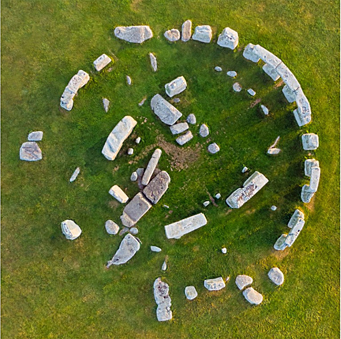
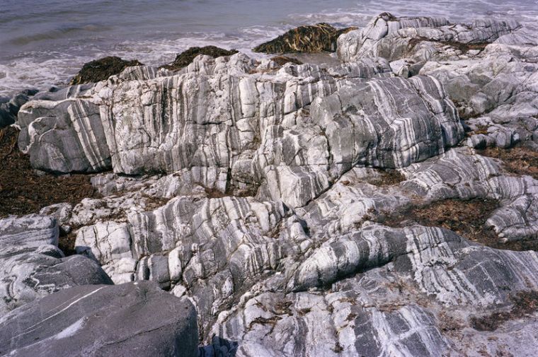
The latest paper examines 13 samples from 8 outcrops of the Middle Devonian Stromness Flagstones strata in the south of the main island of Orkney close to the Ring of Brodgar and the Stones of Stenness, and the individual monoliths in each. On the main island, however, there is a 500 m sequence of Stromness Flagstones in which can be seen 50 cycles of sedimentation. Each cycle contains sandstone beds of various thicknesses and textures. They are fluviatile, lacustrine or aeolian in origin. So the Neolithic builders of Orkney had a wide choice, depending on where they erected monumental structures. Almost certainly they chose monolithic stones where they were most easy to find: close to the coast where exposure can be 100 %. The Ring of Brodgar and the Stones of Stenness are not on the coast, so the enormous stones would have to be dragged there. There is an ancient pile of stones (Vestra Fiold) about 20 km to the NW where some of the mmegaliths may have been extracted, but ancient Orcadians would have been spoilt for choice if they had their hearts set on erecting monoliths!
In a nutshell, the geological case made by Bevins et al. (2024) for rejecting Orkney as the source for the Stonehenge Altar Stone (AS) is as follows: 1. Grains of the mineral baryte (BaSO4) present in the AS are only found in two of the Orkney rock samples. 2. All the Orcadian sandstone samples contain lots of grains of K-feldspar (KAlSi3O8) – common in the basement rocks of northern Scotland – but the AS contains very little. 3. A particular clay mineral (tosudite) is plentiful in the AS, but was not detected in the rock samples from Orkney. Does that rule out a source in Orkney altogether? Well, no: only the outcrops and megalith samples involved in the study are rejected.
To definitely negate an Orcadian source would require a monumental geochemical and mineralogical study across Orkney; covering every sedimentary cycle. Searching the rest of the Old Red Sandstone elsewhere in NE Scotland – and there is a lot of it – would be even more likely to be fruitless. Tracking down the source for the basaltic bluestones at Stonehenge was easy by comparison, because they crystallised from a particular magma over a narrow time span and underwent a specific degree of later metamorphism. They were easily matched visually and under the microscope with outcrops in West Wales in the 1920s and later by geochemical features common to both.
But all that does not detract from the greater importance of the earlier paper (Clarke et al., 2024), which enhanced the idea of Neolithic cultural coherence and cooperation across the whole of Britain. The building of Stonehenge drew people from the far north of Scotland together with those of what are now Wales and England. Since then it hasn’t always been such an amicable relationship …
See also: Addley, E. 2024. Stonehenge tale gets ‘weirder’ as Orkney is ruled out as altar stone origin. The Guardian 5 September 2024.