Photosynthesis, arsenic and a window on the Archaean world

At the very base of the biological pyramid life is far simpler than that which we can see.  It takes the form of single cells that lack a nucleus and propagate only by cloning: the prokaryotes as opposed to eukaryote life such as ourselves. It is almost certain that the first viable life on Earth was prokaryotic, though which of its two fundamental divisions – Archaea or Bacteria – came first is still debated. At present, most prokaryotes metabolise other organisms’ waste or dead remains: they are heterotrophs (from the Greek for ‘other nutrition’). But there are others that are primary producers getting their nutrition by themselves, exploiting the inorganic world in a variety of ways: the autotrophs. Biogeochemical evidence from the earliest sedimentary rocks suggests that, in the Archaean prokaryotic autotrophs were dominant, mainly exploiting chemical reactions to gain energy necessary for building carbohydrates. Some reduced sulfate ions to those of sulphide, others combined hydrogen with carbon dioxide to generate methane as a by-product. Sunlight being an abundant energy resource in near-surface water, a whole range of prokaryotes exploit its potential through photosynthesis. Under reducing conditions some photosynthesisers convert sulfur to sulfuric acid , yet others combine photosynthesis with chemo-autotrophy. Dissolved material capable of donating electrons – i.e. reducing agents – are exploited in photosynthesis: hydrogen, ferrous iron (Fe2+), reduced sulfur, nitrite, or some organic molecules. Without one group, which uses photosynthesis to convert CO2 and water to carbohydrates and oxygen, eukaryotes would never have arisen, for they depend on free oxygen. A transformation 2400 Ma ago marked a point in Earth history when oxygen first entered the atmosphere and shallow water (see: Massive event in the Precambrian carbon cycle; January, 2012), known as Great Oxygenation Event (GOE). It has been shown that the most likely sources of that excess oxygen were extensive bacterial mats in shallow water made of photosynthesising blue-green bacteria that produced the distinctive carbonate structures known as stromatolites. These had formed in Archaean sedimentary basins for 1.9 billion years. It has been generally assumed that blue-green bacteria had formed them too, before the oxygen that they produced overcame the reducing conditions that had generally prevailed before the GOE. But that may not have been the case …

Microbial mats made by purple sulfur bacteria in highly toxic spring water flowing into a salt-lake in northern Chile. (credit: Visscher et al. 2020; Fig 1c)

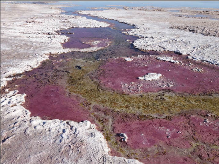
Prokaryotes are a versatile group and new types keep turning up as researchers explore all kinds of strange and extreme environments, for instance: hot springs; groundwater from kilometres below the surface and highly toxic waters. A recent surprise arose from the study of anoxic springs laden with dissolved salts, sulfide ions and arsenic that feed parts of hypersaline lakes in northern Chile (Visscher, P.T. and 14 others 2020. Modern arsenotrophic microbial mats provide an analogue for life in the anoxic ArcheanCommunications Earth & Environment, v. 1, article 24; DOI: 10.1038/s43247-020-00025-2). This is a decidedly extreme environment for life, as we know it, made more challenging by its high altitude exposure to high UV radiation. The springs’ beds are covered with bright-purple microbial mats. Interestingly the water’s arsenic concentration varies from high in winter to low in summer, suggesting that some process removes it, along with sulfur, according to light levels: almost certainly the growth and dormancy of mat-forming bacteria. Arsenic is an electron donor capable of participating in photosynthesis that doesn’t produce oxygen. The microbial mats do produce no oxygen whatever – uniquely for the modern Earth – but they do form carbonate crusts that look like stromatolites. The mats contain purple sulfur bacteria (PSBs) that are anaerobic photosynthesisers, which use sulfur, hydrogen and Fe2+ as electron donors. The seasonal changes in arsenic concentration match similar shifts in sulfur, suggesting that arsenic is also being used by the PSBs. Indeed they can, as the aio gene, which encodes for such an eventuality, is present in the genome of PSBs.

Pieter Visscher and his multinational co-authors argue for prokaryotes similar to modern PSBs having played a role in creating the stromatolites found in Archaean sedimentary rocks. Oxygen-poor, the Archaean atmosphere would have contained no ozone so that high-energy UV would have bathed the Earth’s surface and its oceans to a considerable depth. Moreover, arsenic is today removed from most surface water by adsorption on iron hydroxides, a product of modern oxidising conditions (see: Arsenic hazard on a global scale; May 2020): it would have been more abundant before the GOE. So the Atacama springs may be an appropriate micro-analogue for Archaean conditions, a hypothesis that the authors address with reference to the geochemistry of sedimentary rocks in Western Australia deposited in a late-Archaean evaporating lake. Stromatolites in the Tumbiana Formation show, according to the authors, definite evidence for sulfur and arsenic cycling similar to that in that Atacama springs. They also suggest that photosynthesising blue-green bacteria (cyanobacteria) may not have viable under such Archaean conditions while microbes with similar metabolism to PSBs probably were. The eventual appearance and rise of oxygen once cyanobacteria did evolve, perhaps in the late-Archaean, left PSBs and most other anaerobic microbes, to which oxygen spells death, as a minority faction trapped in what are became ‘extreme’ environments when long before they ‘ruled the roost’. It raises the question, ‘What if cyanobacteria had not evolved?’. A trite answer would be, ‘I would not be writing this and nor would you be reading it!’. But it is a question that can be properly applied to the issue of alien life beyond Earth, perhaps on Mars. Currently, attempts are being made to detect oxygen in the atmospheres of exoplanets orbiting other stars, as a ‘sure sign’ that life evolved and thrived there too. That may be a fruitless venture, because life happily thrived during Earth’s Archaean Eon until its closing episodes without producing a whiff of oxygen.

See also: Living in an anoxic world: Microbes using arsenic are a link to early life. (Science Daily, 22 September 2020)

Did early humans learn to cook in Olduvai Gorge?

Olduvai Gorge in northern Tanzania was for many years the stamping ground of the famous Leakey family and many other anthropologists because of it richness in the skeletal remains and the tools of the earliest members of our genus Homo. The first of these, H. habilis, appears in the Olduvai stratigraphic sequence at around 2 Ma: older examples are now known from localities in Kenya and South Africa taking the species back to about 2.4 Ma. ‘Handy Man’ got the Latinised nickname from its association with abundant stone tools, albeit of a very primitive kind. Oldowan tools are of the ‘let’s bash a couple of pebbles together to get a cutting edge’ kind, dating back to 3.4 Ma (but without evidence of who made them then) and as easily-made disposable tools they linger in the archaeological record until the Neolithic and even modern times. Homo habilis had a brain size little larger than that of australopithecines and some authorities deem them to be such.

Olduvai also yielded the earliest of a more ‘brainy’ species H. ergaster (‘Action Man’), which coexisted with habilis for a few hundred thousand years from around 2 Ma. Initially they also left Oldowan tools. Then, around 1.7 Ma at Olduvai, ergaster began making another stone artefact, the symmetrical bifacial ‘axe’ – probably a multipurpose tool and possibly an object of ritual significance, according to some researchers. Whichever, to make one required visualising the finished item within a shapeless lump of hard rock, and making them required great dexterity: and still does for stone knappers. The biface or ‘Acheulean’ tool originates with one of humanity’s greatest cognitive leaps and lay at the centre of the human toolkit for well over a million years. After being made first in Olduvai by African H. ergaster biface artefacts then spread throughout the continent with H. erectus (probably a direct descendent) and beyond its shores with succeeding humans, up to and including the earliest H. sapiens. How did what seems to be a ‘golden spike’ in human culture first take material form in Olduvai? The possibility of an answer stems from pure serendipity and the development of new research tools.

A flint bifacial stone artefact from the Palaeolithic of Norfolk, UK, which incorporates a bivalve fossil

That the Olduvai Gorge has drawn in several generations of researchers lies in its geology. As well as the sediments deposited by rivers and in ephemeral lakes that characterised a broadly speaking savannah environment, from 2 to 1 Ma there were at least 31 major volcanic eruptions that deposited lavas and a wide range of volcanic ash beds. These have enabled precise dating to calibrate in minute detail the evolution of a highly productive environment and the flora and fauna that it supported during the early Pleistocene. A recently developed technique involves identification of a variety of fatty acids or lipids – natural oils, waxes and steroids – using gas chromatography. Lipids are the remaining ‘biomarkers’ of plants and microorganisms that once lived in an ecosystem. Ainara Sistiaga of the Massachusetts Institute of Technology and the University of Copenhagen, with colleagues from Denmark, Spain, the US and Tanzania, set out to document ecological variation at Olduvai over a million-year interval using this approach. Among the microbial biomarkers they stumbled on something of possibly great importance (Sistiaga, A. and 10 others 2020. Microbial biomarkers reveal a hydrothermally active landscape at Olduvai Gorge at the dawn of the Acheulean, 1.7 Ma. Proceedings of the National Academy of Sciences, v. 117, published online; DOI: 10.1073/pnas.2004532117).

The palaeo-landscape of Olduvai, as revealed by lipid analysis, was highly diverse and rich in grasses, palms shrubs, aquatic flora and edible plants, watered by spring-fed rivers. It supported a diverse fauna including large herbivores (supported by fecal biomarkers): ideal for hominin subsistence. Sistiaga et al. focus in their paper on samples from the 1.7 Ma sedimentary and volcanic sequence (the Lower Augitic Sandstones – augite is an igneous pyroxene) that contains remains of H. ergaster, the oldest bifacial artefacts, and dismembered carcases of hominin prey animals. The surprise that emerged from the volcanoclastic sandstones included lipids produced by a range of bacterial species that only thrive in modern hot springs, such as those at Yellowstone and on the North Island of New Zealand. At three sample sites biomarkers for one particular hyperthermophile were found (Thermocrinis ruber), which can only live in water between 80 to 95°C. This and the other heat-loving bacteria also require water chemistry that, if cool, is drinkable.

Artist’s impression of Homo ergaster cooking an antelope in a 1.7 Ma hot spring at Olduvai Gorge, Tanzania (credit: Tom Björklund, MIT)

The implication is obvious: the ancient Olduvai hot springs were capable of thoroughly cooking meat and vegetables. The importance for humans is that cooking both tenderises meat and tough tubers and roots and breaks down carbohydrates and proteins to make them more easily and efficiently digestible. The brain capacity of H. ergaster was significantly greater than that of H. habilis, and at the average 800 cm3 about 2/3 that of anatomically modern humans. An increase in the input of easily digested protein, fats and carbohydrates may have fuelled that growth and, in turn, the cognitive capacity of H. ergaster. Not only the Western Rift Valley of Tanzania but the whole of the East African Rift System is liberally dotted with hydrothermal vents and also with hominin-rich sites.

See also: Chu, J. 2020. Did our early ancestors boil their food in hot springs? (MIT News, 15 September 2020)

End-Triassic mass extinction: evidence for oxygen depletion on the ocean floor

For British geologists of my generation the Triassic didn’t raise our spirits to any great extent. There’s quite a lot of it on the British Geological Survey 10-miles-to-the-inch geological map (South Sheet) but it is mainly muds, sandstones or pebble beds, generally red and largely bereft of fossils. For the Triassic’s 50 Ma duration following the end-Permian extinction at 252 Ma Britain was pretty much a desert in the middle of the Pangaea supercontinent. Far beyond our travel grants’ reach, the Triassic is a riot, as in the Dolomites of Northern Italy. Apart from a day trip to look at the Bunter Pebble Beds in a quarry near Birmingham and several weeks testing the load-bearing strength of the Keuper mudstones in the West Midlands (not far off zero) in a soil-mechanics lab, we did glimpse the then evocatively named Tea Green Marl (all these stratigraphic names have vanished). Conveniently they outcrop by the River Severn estuary, below its once-famous suspension bridge and close-by the M5 motorway. Despite the Tea Green Marl containing a bone bed with marine reptiles, time didn’t permit us to fossick, and, anyway, there was a nearby pub … The formation was said to mark a marine transgression leading on to the ‘far more interesting Jurassic’ – the reason we were in the area. We were never given even a hint that the end of the Triassic was marked by one of the ‘Big Five’ mass extinctions: such whopping events were not part of the geoscientific canon in the 1960s.

Pangaea just before the start of Atlantic opening at the end of the Triassic, showing the estimated extend of the CAMP large igneous province. The pink triangles show the sites investigated by He and colleagues.

At 201.3 Ma ago around 34 % of marine genera disappeared, comparable with the effect of the K-Pg extinction that ended the Mesozoic Era. Extinction of Triassic terrestrial animals is less quantifiable. Early dinosaurs made it through to diversify hugely during the succeeding Jurassic and Cretaceous Periods. Probably because nothing famous ceased to be or made its first appearance, the Tr-J mass extinction hasn’t captured public attention in the same way as those with the K-Pg or the P-Tr acronyms.  But it did dramatically alter the course of biological evolution. The extinctions coincided with a major eruption of flood basalts known as the Central Atlantic Magmatic Province (CAMP), whose relics occur on either side of the eponymous ocean, which began to open definitively at about the same time. So, chances are, volcanic emissions are implicated in the extinction event, somehow (see: Is end-Triassic mass extinction linked to CAMP flood basalts? June 2013). Tianchen He  of Leeds University, UK and the China University of Geosciences and British and Italian colleagues have studied three Tr-J marine sections on either side of Pangaea: in Sicily, Northern Ireland and British Columbia (He, T. and 12 others 2020. An enormous sulfur isotope excursion indicates marine anoxia during the end-Triassic mass extinction. Science Advances, v. 6, article eabb6704; DOI: 10.1126/sciadv.abb6704). Their objective was to test the hypothesis that CAMP resulted in an episode of oceanic anoxia that caused the many submarine organisms to become extinct. Since eukaryote life depends on oxygen, a deficit would put marine animals of the time under great stress. Such events in the later Mesozoic account for global occurrences of hydrocarbon-rich, black marine shales – petroleum source rocks – in which hypoxia thwarted complete decay of dead organisms over long periods. However there is scant evidence for such rocks having formed ~201 Ma ago. Such as there is dates to about 150 ka younger than the Tr-J boundary in an Italian shallow marine basin. The issue of evidence is compounded by the fact that there are no ocean-floor sediments as old as that, thanks to their complete subduction as Pangaea broke apart in later times and its continental fragments drifted to their present configuration.

But there is an indirect way of detecting deep-ocean anoxia, in the inevitable absence of any Triassic and early Jurassic oceanic crust. It emerges from what happens to the stable isotopes of sulfur when there are abundant bacteria that use the reduction of sulfate (SO42-) to sulfide (S2-) ions. Such microorganisms thrive in anoxic conditions and produce abundant hydrogen sulfide, which in turn leads to the precipitation of dissolved iron as minute grains of pyrite (FeS2). This biogenic process selectively excludes 34S from the precipitated pyrite. As a result, at times of widespread marine reducing conditions seawater as a whole becomes enriched in 34S relative to sulfur’s other isotopes. The enrichment is actually expressed in the unreacted sulfate ions, and they may be precipitated as calcium sulfate or gypsum (CaSO4) in marine sediments deposited anywhere: He et al. focussed on such fractionation. They discovered large ‘spikes’ in the relative enrichment of 34S at the Tr-J boundary in shallow-marine sedimentary sequences exposed at the three sites. Moreover, they were able to estimate that the conditions on the now vanished bed of the Triassic ocean that gave rise to the spikes lasted for about 50 thousand years. The lack of dissolved oxygen resulted in a five-fold increase in pyrite burial in the now subducted ocean-floor sediments of that time. The authors suggest that the oxygen depletion stemmed from extreme global warming, which, in turn, encouraged methane production by other ocean-floor bacteria and, in a roundabout way, other chemical reactions that consumed free dissolved oxygen. Quite a saga of a network of interactions in the whole Earth system that may hold a dreadful warning for the modern Earth and ourselves.

Diamonds and the deep carbon cycle

When considering the fate of the element carbon and CO2, together with all their climatic connotations, it is easy to forget that they may end up back in the Earth’s mantle from which they once escaped to the surface. In fact all geochemical cycles involve rock, so that elements may find their way into the deep Earth through subduction, and they could eventually come out again: the ‘logic’ of plate tectonics. Teasing out the various routes by which carbon might get to mantle is not so easily achieved. Yet one of the ways it escapes is through the strange magma that once produced kimberlite intrusions, in the form of pure-carbon crystals of diamond that kimberlites contain. A variety of petrological and geochemical techniques, some hinging on other minerals that occur as inclusions, has allowed mineralogists to figure out that diamonds may form at depths greater than about 150 km. Most diamonds of gem quality formed in unusually thick lithosphere beneath the stable, and relatively cool blocks of ancient continental crust known as cratons, which extends to about 250 km. But there are a few that reflect formation depths as great as 800 km that span two major discontinuities in the mantle (at 410 and 660 km depth). These transition zones are marked by sudden changes in seismic speed due to pressure-induced transformations in the structure and density of the main mantle mineral, olivine.

Diamond crystal containing a garnet and other inclusions (Credit: Stephen Richardson, University of Cape Town, South Africa)

Carbon-rich rocks that may be subducted are not restricted to limestones and carbon-rich mudstones. Far greater in mass are the basalts of oceanic crust. Not especially rich in carbon when they crystallised as igneous rocks, their progress away from oceanic spreading centres exposes them to infiltration by ocean water. Once heated, aqueous fluids cause basalts to be hydrothermally altered. Anhydrous feldspars, pyroxenes and olivines react with the fluids to break down to hydrated-silicate clays and dissolved metals. Dissolved carbon dioxide combines with released calcium and magnesium to form pervasive carbonate minerals, often occupying networks of veins. So there has been considerable dispute as to whether subducted sediments or igneous rocks of the oceanic crust are the main source of diamonds. Diamonds with gem potential form only a small proportion of recovered diamonds. Most are only saleable for industrial uses as the ultimate natural abrasive and so are cheaply available for research. This now centres on the isotopic chemistry of carbon and nitrogen in the diamonds themselves and the various depth-indicating silicate minerals that occur in them as minute inclusions, most useful being various types of garnet.

The depletion of diamonds in ‘heavy’ 13C once seemed to match that of carbonaceous shales and the carbonates in fossil shells, but recent data from carbonates in oceanic basalts reveals similar carbon, giving three possibilities. Yet, when their nitrogen-isotope characteristics are taken into account, even diamonds that formed at lithospheric depths do not support a sedimentary source (Regier, M.E. et al. 2020. The lithospheric-to-lower-mantle carbon cycle recorded in superdeep diamonds. Nature, v. 585, p. 234–238; DOI: 10.1038/s41586-020-2676-z). That leaves secondary carbonates in subducted oceanic basalts as the most likely option, the nitrogen isotopes more reminiscent of clays formed from igneous minerals by hydrothermal processes than those created by weathering and sedimentary deposition. However, diamonds with the deepest origins – below the 660 km mantle transition zone – suggest yet another possibility, from the oxygen isotopes of their inclusions combined with those of C and N in the diamonds. All three have tightly constrained values that most resemble those from pristine mantle that has had no interaction with crustal rocks. At such depths, unaltered mantle probably contains carbon in the form of metal alloys and carbides. Regier and colleagues suggest that subducted slabs reaching this environment – the lower mantle – may release watery fluids that mobilise carbon from such alloys to form diamonds. So, I suppose, such ultra-deep diamonds may be formed from the original stellar stuff that accreted to form the Earth and never since saw the ‘light of day’.

Monitoring ground motions with satellite radar

By using artificially generated microwaves to illuminate the Earth’s surface it is possible to create images. The technology and the theory behind this radar imaging are formidable. After about 30 years of development using aircraft-mounted transmission and reception antennas, the first high resolution images from space were produced in the late 1970s. Successive experiments improved and expanded the techniques, and for the last decade radar surveillance has been routine from a number of orbiting platforms. Radar has two advantages over optical remote sensing: being an active system it can be done equally effectively day or night; it also penetrates cloud cover, which is almost completely transparent to microwaves with wavelengths between a centimetre and a metre. The images are very different from those produced by visible or infrared radiation, the energy returns from the surface being controlled by topography and the roughness of the surface. One of many complicating factors is that images can only be produced by oblique illumination.  That, together with deployment of widely separated transmission and reception antennas, opens up the possibility of extracting very-high precision (millimetre) measurements of topographic elevation.

In 1992 radar data from two overpasses of the European ERS-1 satellite over California were processed to capture interference due to changes in the ground elevation during the time between the two orbits: the first interferometric radar or InSAR. It revealed the regional ground motions that resulted from the magnitude 7.3 Landers earthquake at 4:57 am local time on June 28, 1992. For the last decade InSAR has become a routine tool to monitor globally both lateral and vertical ground movements, whether rapid, as in earthquakes, or slow in the case of continental plate motions, subsidence or the inflation of volcanoes prior to eruptions. Juliet Biggs and Tim Wright, respectively of the Universities of Bristol and Leeds, UK, have summarised InSAR’s potential (Biggs, J. & Wright, T.J. 2020. How satellite InSAR has grown from opportunistic science to routine monitoring over the last decade. Nature Communications, v. 11, p. 1-4; DOI: 10.1038/s41467-020-17587-6).

Ground motions associated with the 2016 Kaiköuea earthquake on the South Island of New Zealand. Each colour fringe represents 11.4 cm of displacement in the radar line-of-sight (LOS) direction. Known faults are shown as thick black lines (Credit: Hamling et al. 2017. Complex multifault rupture during the 2016 Mw 7.8 Kaikōura earthquake, New Zealand. Science, v. 356, article eaam7194; DOI: 10.1126/science.aam7194)

Since the ERS-1 satellite discovered the ground motions associated with the Landers earthquake, InSAR has covered more than 130 large seismic events. Although the data post-dated the damage, they have demonstrated the particular mechanics of each earthquake, allowing theoretical models to be tested and refined. In the image above it is clear that the motions were not associated with a single fault in New Zealand: the Kaikoura earthquake involved a whole network of them, at least at the surface. Probably, displacement jumped from one to another; a complexity that must be taken into account for future events on such notorious fault systems as those in densely populated parts of California and Turkey.

East to west speed of the Anatolian micro-plate south of the North Anatolian Fault derived from the first five years of the EU’s Sentinel-1 InSAR constellation. Major known faults shown by black lines (Credit: Emre, O. et al. 2018. Active fault database of Turkey. Bulletin of Earthquake Engineering, v. 16, p. 3229-3275; DOI: 10.1007/s10518-016-0041-2)

Since its inception, GPS has proved capable of monitoring tectonic motions over a number of years, but only for widely spaced, individual ground instruments. Using InSAR alongside years’ worth of GPS measurements helps to extend detected motions to much finer resolution, as the image above shows for Asiatic Turkey. An important parameter needed for prediction of earthquakes is the way in which crustal strain builds up in regions with dangerously active fault systems.

InSAR image of the Sierra Negra volcano on Isabela Island in the Galapagos Archipelago, at the time of a magma body intruding its flanks. Each colour fringe represents 2.8 cm of subsidence in the LOS direction (Credit: Anantrasirichai, N. et al. 2019. A deep learning approach to detecting volcano deformation from satellite imagery using synthetic datasets. Remote Sensing of Environment, v. 230, article 111179; DOI: 10.1016/j.rse.2019.04.032)

Volcanism obviously involves the movement of large masses of magma beneath the surface before eruptions. GPS and micro-gravity measurements show that charging of a magma chamber causes volcanoes to inflate so InSAR provides a welcome means of detecting the associated uplift, even if it only a few centimetres, as show by the example above from the Galapagos Islands. A volcano’s flanks may bulge, which could presage a lateral eruption or a pyroclastic flow such as that at Mount St Helens in 1980. Truly vast eruptions are associated with calderas whose ring faults may cause collapse in advance.

The presence of cavities beneath the surface, formed by natural solution of limestones, deliberately as in extraction of brines from salt deposits or after subsurface mining, present subsidence hazards. There have been several series of alarming TV programmes about sinkhole formation that demonstrate sudden collapse. Yet every case will have been preceded by years of gradual sagging. InSAR allows risky areas to be identified well in advance of major problems. Indeed estate agents (realtors) as well as planners, civil engineers and insurers form a ready market for such survey.

Natural sparkling water and seismicity

For all manner of reasons, natural springs have fascinated people since at least as long ago as the Neolithic. Just the fact that clear water emerges from the ground to source streams and great rivers seems miraculous. There are many occurrences of offerings having been made to supernatural spirits thought to guard springs. Even today many cannot resist tossing in a coin, hanging up a ring, necklace or strip of cloth beside a spring, for luck if nothing else. Hot springs obviously attract attention and bathers. Water from cool ones has been supposed to have health-giving properties for at least a couple of centuries, even if they stink of rotten eggs or precipitate yellow-brown iron hydroxide slime in the bottom of your cup. Spas now attribute their efficacy to their waters’ chemistry, and that depends on the rocks through which they have passed. Those in areas of volcanic rock are generally the most geochemically diverse: remember the cringe-making adverts for Volvic from the volcanic Chain des Puys in the French Auvergne. Far more ‘posh’ are naturally carbonated waters that well-out full of fizz from pressurised, dissolved CO2. Internationally the best known of these is Perrier from the limestone-dominated Gard region of southern France. Sales of bottled spring waters are booming and the obligatory water-chemistry data printed on their labels form  a do-it-yourself means of regional geochemical mapping (Dinelli, E. et al. 2010. Hydrogeochemical analysis on Italian bottled mineral waters: Effects of geology. Journal of Geochemical Exploration, v. 107, p. 317–335; DOI: 10.1016/j.gexplo.2010.06.004) But it appears from a study of variations in CO2 output from commercial springs in Italy that they may also help in earthquake prediction (Chiodini, G. et al. 2020. Correlation between tectonic CO2 Earth degassing and seismicity is revealed by a 10-year record in the Apennines, Italy. Science Advances, v. 6, article eabc2938; DOI: 10.1126/sciadv.abc2938).

Italy produces over 12 billion litres of spring water and the average Italian drinks 200 litres of it every year. There are more than 600 separate brands of acqua minerale produced in Italy, including acqua gassata (sparkling water). Even non-carbonated springs emit CO2, so it is possible to monitor its emission from the deep Earth across wide tracts of the country. High CO2 emissions are correlated worldwide with areas of seismicity, either associated with shallow magma chambers or to degassing from subduction zones. There are two possibilities: that earthquakes help release built-up fluid pressure or because fluids, such as CO2 somehow affect rock strength. Giovanni Chiodini and colleagues have been monitoring variations in CO2 release from carbonated spring water in the Italian Apennines since 2009. Over a ten-year period there have been repeated earthquakes in the area, including three of magnitude 6.0 or greater. The worst was that affecting L’Aquila in April 2009, the aftermath of which saw six geoscientists charged with – and eventually acquitted of – multiple manslaughter (see: Una parodia della giustizia?, October 2012). It was this tragedy that prompted Chiodini et al.’s unique programme of 21 repeated sampling of gas discharge rates at 36 springs, matched to continuous seismograph records. The year after the L’Aquila earthquake coincided with high emissions, which then fell to about half the maximum level by 2013. In 2015 emissions began to rise to reach a peak before earthquakes with almost the same magnitude, but less devastation, on 24 August and 30 October 2016. Thereafter emissions fell once again. This suggests a linked cycle, which the authors suggest is modulated by ascent of CO2 that originates from the melting of carbonates along the subduction zone that dips beneath central Italy. They suggest that gas accumulates in the lower crust and builds up pressure that is able to trigger earthquakes in the crust.

The variation in average emissions across central Italy (see figure above) suggests that there are two major routes for degassing from the subduction zone, perhaps focussed by fractures generated by previous crustal tectonic movements. In my opinion, this study does not prove a causal link, although that is a distinct possibility, which may be verified by extending this survey of degassing and starting similar programmes in other seismically active areas. Whether or not it might become a predictive tool depends on further work. However, other studies, particularly in China, show that other phenomena associated with groundwater in earthquake-prone areas, such as rise in well-water levels and an increase in their emissions of radon and methane, correlate in a similar manner.