Climate changes and the mass extinction at Permian-Triassic boundary

The greatest mass extinction in Earth’s history at around 252 Ma ago snuffed out 81% of marine animal species, 70% of vertebrates and many invertebrates that lived on land. It is not known how many land plants were removed, but the complete absence of coals from the first 10 Ma of the Early Triassic suggests that luxuriant forests that characterised low-lying humid area in the Permian disappeared. A clear sign of the sudden dearth of plant life is that Early Triassic river sediments were no longer deposited by meandering rivers but by braided channels. Meanders of large river channels typify land surfaces with abundant vegetation whose root systems bind alluvium. Where vegetation cover is sparse, there is little to constrain river flow and alluvial erosion, and wide braided river courses develop (see: End-Permian devastation of land plants; September 2000. You can follow 21st century developments regarding the P-Tr extinction using the Palaeobiology index).

The most likely culprit was the Siberian Trap flood basalts effusion whose lavas emitted huge amounts of CO2 and even more through underground burning of older coal deposits (see: Coal and the end-Permian mass extinction; March 2011) which triggered severe global warming. That, however, is a broad-brush approach to what was undoubtedly a very complex event. Of about 20 volcanism-driven global warming events during the Phanerozoic only a few coincide with mass extinctions. Of those none comes close the devastation of ‘The Great Dying’, which begs the question, ‘Were there other factors at play 252 Ma ago?’ That there must have been is highlighted by the terrestrial extinctions having begun significantly earlier than did those in marine ecosystems, and they preceded direct evidence for climatic warming. Also temperature records – obtained from shifts in oxygen isotopes held in fossils – for that episode are widely spaced in time and tell palaeoclimatologists next to nothing about the details of the variation of air- and sea-surface temperature (SST) variations.

Modelled sea-surface temperatures in the tropics in the early stages of Siberian Trap eruptions with atmospheric CO¬2 at 857 ppm – twice today’s level. (Credit: Sun et al., Fig. 1A)

Earth at the end of the Permian was very different from its current wide dispersal of continents and multiple oceans and seas. Then it was dominated by Pangaea, a single supercontinent that stretched almost from pole to pole, and a surrounding vast ocean known as Panthalassa. Geoscientists from China, Germany, Britain and Austria used this simple palaeogeography and the available Early Triassic greenhouse-gas and  palaeo-temperature data as input to a climate prediction model (HadCM3BL) (Yadong Sun and 7 others 2024. Mega El Niño instigated the end-Permian mass extinction. Science 385, p. 1189–1195; DOI: 10.1126/science.ado2030  – contact yadong.sun@cug.edu.cn for PDF).. The computer model was developed by the Hadley Centre of the UK Met Office to assess possible global outcomes of modern anthropogenic global warming. It assesses heat transport by atmospheric flow and ocean currents and their interactions. The researchers ran it for various levels of atmospheric CO2 concentrations over the estimate 100 ka duration of the P-Tr mass extinction.

The pole-to-pole continental configuration of Pangaea lends itself to equatorial El Niño and El Niña type climatic events that occur today along the Pacific coast of the Americas, known as the El Niño-Southern Oscillation. In the first, warm surface water builds-up in the eastern tropical Pacific Ocean. It then then drifts westwards to allow cold surface water to flow northwards along the Pacific shore of South America to result in El Niña. Today, this climatic ‘teleconnection’ not only affects the Americas but also winds, temperature and precipitation across the whole planet. The simpler topography at the end of the Permian seems likely to have made such global cycles even more dominant.

Sun et al’s simulations used stepwise increases in the atmospheric concentration of CO2 from an estimated  412 parts per million (ppm) before the eruption of the Siberian Traps (similar to those today) to a maximum of 4000 ppm during the late-stage magmatism that set buried coals ablaze. As levels reached 857 ppm SSTs peaked at 2 °C above the mean level during El Niño events and the cycles doubled in length. Further increase in emissions led to greater anomalies that lasted longer, rising to 4°C above the mean at 4000 ppm. The El Niña cooler parts of the cycle steadily became equally anomalous and long lasting. This amplification of the 252 Ma equivalent of the El Niño-Southern Oscillation would have added to the environmental stress of an ever increasing global mean surface temperature.  The severity is clear from an animation of mean surface temperature change during a Triassic ENSO event.

Animation of monthly average surface temperatures across the Earth during an ENSO event at the height of the P-Tr mass extinction. (Credit: Alex Farnsworth, University of Bristol, UK)

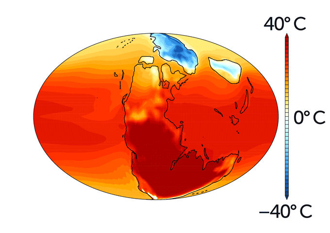
The results from the modelling suggest increasing weather chaos across the Triassic Earth, with the interior of Pangaea locked in permanent drought. Its high latitude parts would undergo extreme heating and then cooling from 40°C to -40°C during the El Niño- El Niña cycles. The authors suggest that conditions on the continents became inimical for terrestrial life, which would be unable to survive even if they migrated long distances. That can explain why terrestrial extinctions at the P-Tr boundary preceded those in the global ocean. The marine biota probably succumbed to anoxia (See: Chemical conditions for the end-Permian mass extinction; November 2008)

There is a timely warning here. The El Niño-Southern Oscillation is becoming stronger, although each El Niño is a mere 2 years long at most, compared with up to 8 years at the height of the P-Tr extinction event. But it lay behind the record 2023-2024 summer temperatures in both northern and southern hemispheres, the North American heatwave of June 2024 being 15°C higher than normal. Many areas are now experiencing unprecedentedly severe annual wildfires. There also finds a parallel with conditions on the fringes of Early Triassic Pangaea. During the early part of the warming charcoal is common in the relics of the coastal swamps of tropical Pangaea, suggesting extensive and repeated wildfires. Then charcoal suddenly vanishes from the sedimentary record: all that could burn had burnt to leave the supercontinent deforested.

See also: Voosen, P. 2024. Strong El Niños primed Earth for mass extinction. Science 385, p. 1151; DOI: 10.1126/science.z04mx5b; Buehler, J. 2024. Mega El Niños kicked off the world’s worst mass extinction. ScienceNews, 12 September 2024.

The end of the Carboniferous ‘icehouse’ world

From about 340 to 290 Ma the Earth experienced the longest episode of repeated ice ages of the Phanerozoic. The climate then was similar in many ways to that of the Pleistocene. The South Polar region was then within the Pangaea supercontinent and thus isolated from any warming effect from the surrounding ocean: much the same as modern Antarctica but on a much larger scale. Glaciation extended as far across what became the southern continents and India as did the continental ice sheets of the Northern Hemisphere during Pleistocene glacial maxima. Tropical sedimentary rocks of the time, display evidence for repeated alternations of high and low sea levels that mark cycles of glacial maxima and interglacial episodes akin to those of the Pleistocene. In fact they probably reflect the influence of changes in the Earth’s orbit and geometry of its axis of rotation very similar to those predicted by Milankovich from astronomical factors to explain Pleistocene climatic cycles. At the end of the Carboniferous what was an ‘ice-house’ world changed suddenly to its opposite – ‘greenhouse’ conditions – that persisted through the Mesozoic Era until the later part of the Cenozoic, when Antarctica developed is ice cap and global climate slowly cooled to become extremely cyclical once again.

Sedimentary evidence for global climates 320 Ma ago. As well as the large tracts of glaciogenic sediments, smaller occurrences and examples of polished rock surfaces over which ice had passed show the probable full extent (blue line) of ice sheets across the southern, Gondwana sector of Pangaea (Credit: after Fig 7.3, S104, Earth and Space, ©Open University 2007)

The end of the Carboniferous witnessed the collapse of the vast Equatorial rainforests, which formed the coal deposits that put ‘Carbon’ into the name of the Period. By its end this ecosystem had vanished to result in a minor mass extinction of both flora and fauna. Temperatures rose and aridity set in, to the extent that the latest Carboniferous in the British coalfields is marked by redbeds that presage the spread of desert conditions across the Equatorial parts of Pangaea during the succeeding Permian. A team of researchers based at the University of California at Davis have been studying data pertaining to this sudden change have now published their findings (Chan J. and 17 others 2022. Marine anoxia linked to abrupt global warming during Earth’s penultimate icehouse. Proceedings of the National Academy of Sciences, v. 119, article e2115231119; DOI: 10.1073/pnas.2115231119). They used carbon-, oxygen- and uranium isotopes, together with proxies for changes in atmospheric CO2 concentrations, to model changes in the carbon cycle in the Late Carboniferous of China.

Changes in uranium isotopes within marine carbonates are useful indicators of the amount of oxygen available in ocean water at the sea floor. Between 304 and 303.5 Ma ago oxygen content declined by around 30%, the peak of this anoxia being at 303.7 Ma. This occurred about 100 ka after atmospheric CO2 had risen to ~700 parts per million (ppm) from around 350 ppm in the preceding 300 ka, as marked by several proxies.  The authors suggest that the lower ‘baseline’ for the main greenhouse gas marked an extreme glacial maximum. Changes in the proportions of 18O relative to ‘lighter’ 16O in fossil shells suggest that sea-surface temperatures increased in step with the doubling of the greenhouse effect. At the same time there was a major marine transgression as sea level rose. This would have been accompanied by a massive increase in low density freshwater in surface ocean water derived from melting of Pangaea’s ice cap. The team suggests that the freshened surface layer could not sink to carry oxygen to deeper levels, thereby creating anoxic conditions across an estimated 23% of the global seafloor, and thus toxic ‘death zones’ for marine organisms.

One possibility for this sudden rise of atmospheric CO2 is a massive episode of volcanism, perhaps a large igneous province, but there is scanty evidence for that at the end of the Carboniferous. A coinciding sharp decrease in δ13C  in carbonate shells suggests that the excess carbon dioxide probably had an organic origin. So a more plausible hypothesis is massive burning on the continental surface. In the tropics, the huge coals swamps would have contained vast amounts of peat-like decayed vegetable matter as well as living green vegetation. How might that have caught fire? The peat precursor to Carboniferous coal deposits derived from photosynthesis on an unprecedented, and never repeated, scale during tens of million years of thriving tropical rain forest during that Period. This built up atmospheric oxygen levels to about 35%, compared with about 21% today. Insects, whose maximum size is governed by their ability to take in oxygen through spiracles in their bodies, and by the atmospheric concentration of oxygen, became truly huge during the earlier Carboniferous. The more oxygen in the air, the greater the chance that organic matter will catch fire. In fact wet vegetation can burn if oxygen levels rise above 25%. At the levels reached in the Carboniferous huge wildfires in forests and peatlands would have been inevitable. Evidence that huge fires did occur comes from the amount of charcoal found in Carboniferous coal seams, which reach 70% compared with the 4 to 8 % in more recent coals. They may have been ignited by lightning strikes or even spontaneous combustion if decay of vegetation generated sufficient heat, as sometimes happens today in wet haystacks or garden compost heaps.  But how in a short period around 304 Ma could 9 trillion tons of carbon dioxide be released in this way. The preceding  glacial super-maximum, like glacial maxima of the Pleistocene, may have been accompanied by decreased atmospheric humidity: this would dry out the vast surface peat deposits.

The succeeding Permian is famous for its extensive continental redbeds, and so too those of the Triassic. They are red because sediment grains are coated in the iron oxide hematite (Fe2O3). As on Mars, the redbeds are a vast repository for oxygen sequestered from the atmosphere by the oxidation of dissolved Fe2+ to insoluble Fe3+. This had been going on throughout the Permian, the nett result being that by 250 Ma atmospheric oxygen content has slumped to 16% and remained so low for another 50 million years. Photosynthesis failed to resupply oxygen against this inorganic depletion, and there are few coal deposits of Permian or Triassic age: for about 100 Ma Earth ceased to have green continents.

See also: Carbon, climate change and ocean anoxia in an ancient icehouse world. Science Daily, 2 May 2022. 

Late Palaeozoic glacial features in Chad

The longest and most extreme glacial epoch during the Phanerozoic took place between 360 and 260 Ma ago, when it dominated the Carboniferous and Permian sedimentary sequences across the planet. On continents that lay athwart the Equator during these times, sedimentation was characterised by cycles between shallow marine and terrestrial conditions. These are epitomised by the recurring ‘Coal-Measure’ cyclothem of, from bottom to top: open-sea limestone; near-shore marine mudstone; riverine sandstone; coal formed in swamps. This sequence represents a rapid rise in sea level as ice sheets melted, sustained during an interglacial episode and then falling sea level as ice once again accumulated on land to culminate in a glacial maximum when coal formed in coastal mires. During the Late Palaeozoic Era a single supercontinent extended from pole to pole. The break-up of Pangaea was charted by Alfred Wegener in 1912, partly by his using glacial deposits and ice-gouged striations on the southern continents. With the present widely separated configuration of major landmasses glacial sediments and the directions of inferred ice movements could only be reconciled by reassembling Africa, India, South America, Antarctica and Australia in the form of a single, congruent southern continent that he called Gondwanaland. In Wegener’s reconstruction the glacial features massed together on Gondwanaland with the striations radiating outwards from what would then have been the centre of a huge ice cap.

There are many localities on the present southern continents where such striations can be seen on the surface of peneplains etched into older rocks that underlie Carboniferous to Permian tillites, but later erosion has removed the continuity of the original glacial landscape. There are, however, some parts of central Africa where it is preserved. By using the high-resolution satellite images (with pixels as small as 1 m square) that are mosaiced together in Google Earth, Daniel Paul Le Heron of Royal Holloway, University of London has revealed a series of 1 to 12 km wide sinuous belts in a 6000 km2 area of eastern Chad that are superimposed unconformably on pre-Carboniferous strata (Le Heron, D.P. 2018. An exhumed Paleozoic glacial landscape in Chad. Geology, v.46(1), p. 91-94; doi:10.1130/G39510.1). They comprise irregular tracts of sandstone to the south of a major Carboniferous sedimentary basin. Zooming in to them (try using 17.5° N 22.25°E as a search term in Google Earth) reveals surfaces dominated by wavy, roughly parallel lines. Le Heron interprets these as mega-scale glacial lineations, formed by ice flow across underlying soft Carboniferous glacial sediments as seen in modern glacial till landforms in Canada. In places they rest unconformably on older rocks, sometimes standing above the level of the sandstone plateaux as relics of what may have been nunataks. There are even signs of elliptical drumlins.

An oblique Google Earth view looking to the south-east shows mega-scale glacial lineations from a glacial flow way in eastern Chad. The lower-right quadrant shows the unconformity atop older bedded strata that are dipping to the west. Click on the image to see a full resolution view. (Credit: Google Earth)

Glacial tillites and glaciofluvial sediments of Late Palaeozoic age are common across the Sahara and in the Sahelian belt, but in areas as remote as those in eastern Chad. So a systematic survey using the resolving power of Google Earth may well yield yet more examples. It is tedious work in such vast areas, unless, of course, one bears in mind Alfred Wegener, the founder of the hypothesis of continental drift and ‘Big’ Earth Science as a whole, who would have been gleeful at the opportunity.

A fully revised edition of Steve Drury’s book Stepping Stones: The Making of Our Home World can now be downloaded as a free eBook

Yes, it was hot during the Permian

For those of us living in what was the heart of Pangaea – Europe and North America – more than 250 Ma ago this item’s title might seem like the ultimate truism. However, despite our vision of desert dune sands and evaporating inland seas, glaciation blanketed much of the Gondwana part of the supercontinent until the Middle Permian then lying athwart the South Pole. That would go a long way to accounting for extreme dryness at low to mid-latitudes, especially in the deep interior of Pangaea, but just how hot might tropical climates have been? The deglaciation of Gondwana was abrupt and has been touted as an analogue for a possible anthropogenic closure to the Cenozoic glacial epoch that began around 34 Ma in Antarctica and has periodically gripped land at northern latitudes as low as 40°N for the last 2.5 Ma. Since the present distribution of continents is totally different from the unique pole-to-pole shape of Pangaea, that is probably a view that is not widely held by palaeoclimatologists. Nonetheless, getting hard data on Permian conditions has an intrinsic interest for most geoscientists.

The bottom of Death Valley, USA
Playa lake in Death Valley, USA (credit: Wikipedia)

One of the best ways of measuring past temperatures, whether surficial or deep within the crust, almost directly is based on fluids trapped within minerals formed at the time of interest. In Permian strata there is no shortage of suitable material in the form of evaporite minerals, especially common salt or halite.  A distinctive chevron-like texture develops in halite that forms at the water-atmosphere interface in playa lakes that dry out every year. When thin sections of samples that contain fluid inclusions are slowly heated the air bubbles trapped in salt during crystallisation gradually homogenise with the other trapped fluids. Based on samples that have formed at the present day under a range of air temperatures, the temperature of homogenisation indicates the prevailing air temperature accurately. So well, in fact, that it is possible to assess diurnal temperature variations in suitable halite crystals.

Results have been obtained from Middle Permian halites in Kansas, USA (Zambito, J.J. & Benison, K.C. 2013. Extremely high temperatures and paleoclimate trends recorded in Permian ephemeral lake halite. Geology, v. 41, p. 587-590). In part of the section studied air temperatures reached 73°C, compared with a modern maximum of 57°C recorded in halites from the playas of Death Valley. Moreover, they exhibit changes of more than 30°C during daily cycles. But that kind of weather is common in other hot dry areas today, such as the Dasht-e Lut in eastern Iran. Also, the full data show crystallisation at lower temperatures (maxima of 30-40°C) in part of the sequence. What is noteworthy is that these data are the first quantitative indicators of weather before the last 2.5 Ma. Since evaporites extend back into the Precambrian, the method will undoubtedly extend accuracy and precision to paleoclimate  where only proxies and a modicum of guesswork were previously available.