When the Arctic Ocean was filled with fresh water

The salinity of surface water at high latitudes in the North Atlantic is a critical factor in its sinking to draw warm, low-latitude water northwards in the Gulf Stream while contributing to the southwards flow of North Atlantic Deep Water along the ocean floor. One widely supported hypothesis for rapid cooling events, such as the Younger Dryas, is the shutdown of this thermohaline circulation (Review of thermohaline circulation, February 2002). That may happen when surface seawater at high latitudes is freshened and made less dense by rapid melting or break-up of continental ice sheets, or through the release of vast amounts of fresh water from glacially dammed lakes. The climatic decline leading to the last glacial maximum at around 20 ka was punctuated by irregular episodes known as Dansgaard-Oeschger and Heinrich Events that have been attributed to such hiccups in thermohaline processes. In this context, a whole new barrel of fish has been opened up by a geochemical study of the top few metres of sediments on the Arctic Ocean floor (Geibert, W. et al. 2021. Glacial episodes of a freshwater Arctic Ocean covered by a thick ice shelfNature, v. 590, p. 97–102; DOI: 10.1038/s41586-021-03186-y), particularly their content of an isotope of thorium (230Th).

Being radioactive (half-life ~75 ka), 230Th is useful in working out sediment deposition rates, especially as it is insoluble and adheres to dust grains. The isotope is a decay product of uranium, yet it not only forms on land from uranium in hard rocks, eventually to be transported into marine sediments, but from uranium dissolved in seawater too. Interestingly, the amount of uranium that can enter seawater in solution depends on water salinity. Fresh water, especially that locked up in glacial ice, has very low concentrations of uranium. Consequently, ordinary seawater adds additional 230Th to sediments whereas fresh water does not. An excess of the isotope in marine sediments signifies their deposition from salty water, but those deposited in fresh water carry no excess. In the course of analysing deep-sea cores from the floors of the Arctic Ocean and the northernmost part of the North Atlantic, Walter Geibert and colleagues at the Alfred Wegener Institute in Bremerhaven, and the University of Bremen, Germany revealed a series of sediment layers that were devoid of excess 230Th. This suggests that twice, probably in periods between 150 to 131 and 70 to 62 ka, water in the Arctic Ocean and the connected Nordic Sea was entirely fresh. In two cores the evidence suggests a third, restricted occurrence of fresh water fill at about 15 ka.

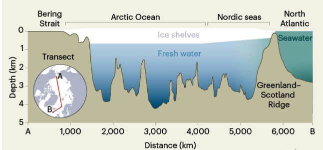
The most likely explanation is that the fresh-water episodes marked the development of major ice shelves, similar to those still present around Antarctic; i.e. floating or grounded ice of glacial origin (not sea ice). That had been anticipated, but not previously proved for the northern polar region. The outlets from the Arctic Ocean basin to the Pacific and North Atlantic Oceans are marked by barriers of shallow seabed. One is the Bering Straits, which became the Beringia land bridge that facilitated animal and human migrations from Siberia to North America when sea level fell as continental ice sheets grew. The other is the Greenland-Scotland Ridge formed by volcanism connected to the Icelandic hot spot as the North Atlantic opened. It is possible that the suggested ice shelves grounded on these ridges, to effectively dam and isolate the Arctic Ocean. Fresh water from melting land ice would ‘pond’ beneath the ice shelves, floating on denser salt water and eventually expelling it from much of the polar marine basin. A side effect of this would have been partially to accumulate and isolate the oxygen-isotope proportions that characterise snow and glacial ice. Remember that the light 16O isotope is preferentially extracted from sea water during evaporation, to become stored in glacial ice sheets so that the proportion of the heavier 18O increases in ocean water; δ18O is therefore an important proxy for glacial waxing and waning and thus the fluctuations of global sea level. Trapping a proportion of water of glacial origin in isolated Arctic Ocean water and ice shelves would explain discrepancies in the oxygen-isotope records of successive ice ages. Also, if the ice shelves periodically broke up, fresh water derived from them and ponded in the deepest Arctic Ocean basin could change the salinity of surface ocean water elsewhere – being lower density that fresh water would ‘float’.

The work of Geibert and colleagues may well result in a great deal of head scratching among palaeoclimatologists and perhaps new ideas on the dynamics of ice age climates.

See also: Hoffmann, S. 2021. The Arctic Ocean might have been filled with freshwater during ice ages. Nature, v. 590, p. 37-38; DOI: 10.1038/d41586-021-00208-7

Odds and ends about Milankovitch and climate change

It is some 40 years since the last explosive development in understanding the way the world works. In 1976 verification of Milutin Milanković’s astronomical theory to explain cyclical climate change as expressed by surface processes has had a similar impact as the underpinning of internal processes by the emergence of plate tectonics in the preceding decade. Signals that match the regularity of changes in the Earth’s orbital eccentricity and the tilt and precession of its axis of rotation, with periods of roughly 96 and 413 ka, 41 ka, 21 and 26 ka respectively, were found in climate change proxies in deep-sea sediment cores (oxygen isotope sequences from benthonic foraminifera) spanning the last 2.6 Ma. The findings seemed as close to proof as one might wish, albeit with anomalies. The most notable of these was that although Milanković’s prediction of a dominant 41 ka effect of changing axial tilt, the strongest astronomical forcing, had characterised cooling and warming cycles in the early Pleistocene, since about a million years ago a ~100 ka periodicity took over – that of the weakest forcing from changing orbital obliquity. Analysis of sedimentary cycles from different episodes in earlier geological history, as during Carboniferous to Permian global frigidity, seemed to confirm that gravitational fluctuations stemming from the orbits of other planets, Jupiter and Saturn especially, had been a continual background to climate change.

All manner of explanations have been offered to explain why tiny, regular and predictable changes in Earth’s astronomical behaviour produce profound changes in the highly energetic and chaotic climate system. Much attention has centred on the mathematically based concept of stochastic resonance. That is a phenomenon where weak signals may be induced to show themselves if they are mixed with a random signal – ‘white noise’ spanning a great range of frequencies. The two resonate at the hidden frequencies thereby strengthening the weak, non-random signal. Noise is already present in the climate system because of the random and highly complex nature of the components of climate itself and the surface processes that it induces.

The latest development along these lines suggests that something quite simple may be at the root of inner complexities in the climatic history of the Pleistocene Epoch: the larger an ice sheet becomes and the longer it lasts the easier it is to cause it to melt away (Tzedakis, P.C. et al. 2017. A simple rule to determine which insolation cycles lead to interglacials. Nature, v. 542, p. 427-432; doi:10.1038/nature21364). The gist of the approach taken in the investigation lies in analysing the degree to which the onsets of major ice-cap melting match astronomically predicted peaks in summer insolation north of 65° N. It also subdivides O-isotope signals of periods of sea level rise into full interglacials, interstadials during periods of climate decline and a few cases of extended interglacials. Through time it is clear that there has been an  increase in the number of interstadials that interrupt cooling between interglacials. Plotting the time of peaks in predicted summer warming closest to major glacial melting events against their insolation energy is revealing.

Before 1.5 Ma the peak energy of summer insolation in the Northern Hemisphere exceeded a threshold leading to full interglacials rather than interstadials more often than it did during the period following 1 Ma. Although Milanković’s 41 ka periodicity remained recognisable throughout, from about 1.5 Ma ago more and more of the energy peaks resulted in only the partial ice melting of interstadial events. The energy threshold for the full deglaciation of interglacials seems to have increased between 1.5 to 1.0 Ma and then settled to a ‘steady state’. The balance between glacial growth and melting increasingly ‘skipped’ 41 ka peaks in insolation so that ice caps grew bigger with time. Deglaciation then required additional forcing. But considering the far larger extent of ice sheets, the tiny additional insolation due to shifts in  orbital eccentricity every ~100 ka surprisingly tipped truly savage ice ages into warm interglacials.

Resolving this paradox may lie with three simple, purely terrestrial factors associated with great ice caps: thicker and more extensive ice becomes warmer at its base and more prone to flow; climate above and around large ice caps becomes progressively colder and drier, so reducing their growth rate; the more sea level falls as land ice builds up, the more the vertical structure and flow of ocean water change. The first of these factors leads to periodic destabilisation when ice sheets surge outwards and increase the rate of iceberg calving into the surrounding oceans. Such ‘iceberg armadas’ characterised the last Ice Age to result in sudden irregularly spaced changes in ocean dynamics and global climate to return to metastable ice coverage, as did earlier ones of similar magnitude. The second factor results in dust lingering at the surface of ice caps that reduced the ability of ice to reflect solar radiation back to space, which enhances summer melting. The third and perhaps most profound factor reduces the formation of ocean bottom water into which dissolved carbon dioxide has accumulated from thermohaline sinking of surface water. This leads to more CO2 in the atmosphere and a growing greenhouse effect. Comforting as finding simplicity within huge complexity might seem, that orbital eccentricity’s weak effect on climatic warming – an order of magnitude less than any other astronomical forcing – can tip climate from one extreme to the other should be a grave warning: climate is chaotic and responds unpredictably to small changes …

Snowball Earth events pinned down

The Period that lasted from 850 to 635 million years ago, the Cryogenian, takes its name from evidence for two and perhaps three episodes of glaciation at low latitudes. It has been suggested that, in some way, they were instrumental in the decisive stage of biological evolution from which metazoan eukaryotes emerged: the spectacular Ediacaran fossil assemblages follow on the heels of the last such event Although controversies about the reality of tropical latitudes experiencing ice caps have died away, there remains the issue of synchronicity of such frigid events on all continents, which is the central feature of so-called ‘Snowball Earth’ events. While each continent does reveal evidence for two low latitude glaciations – the Sturtian (~710 Ma) and the later Marinoan (~635 Ma) – in the form of diamictites (sediments probably dropped from floating ice and ice caps) it has proved difficult to date their start and duration. That is, the cold episodes may have been diachronous – similar conditions occurring at different localities at different times. Geochronology has, however, moved on since the early disputes over Snowball Earths and more reliable and precise dates for beginnings and ends are possible and have been achieved in several places (Rooney, A.D. et al. 2015. A Cryogenian chronology: Two long-lasting synchronous Neoproterozoic glaciations. Geology, v. 43, p. 459-462).

One computer simulation of conditions during a...
Computer simulation of conditions during a Snowball Earth period. (credit: Macmillan Publishers Ltd: Hyde et al., Nature 405:425-429, 2000)

Rooney and colleagues from Harvard and the University of Houston in the USA used rhenium-osmium radiometric dating in Canada, Zambia and Mongolia. The Re-Os method is especially useful for sulfide minerals as in the pyritic black shales that occur extensively in the Cryogenian, generally preceding and following the glacial diamictites and their distinctive carbonate caps. Combined with a few ages obtained by other workers using the Re-Os method and U-Pb dating of volcanic units that fortuitously occur immediately beneath or within diamictites, Rooney et al. establish coincident start and stop dates and thus durations of both the Sturtian and Marinoan glacial events: 717 to 660 Ma and 640 to 635 Ma respectively on all three continents. Their data is also said to refute the global extent and even the very existence of an earlier, Kaigas glacial event (~740 Ma) previous recorded from diamictites in Namibia, the Congo, Canada and central Asia. This assertion is based on the absence of diamictites with that age in the area that they studied in Canada and their own dating of a diamictite in Zambia, which is one that others assigned to the Kaigas event

The dating is convincing evidence for global glaciation on land and continental margins in the Cryogenian, as all the dates are from areas based on older continental crust. But the concept of Snowball Earth, in its extreme form, is that the oceans were ice-capped too as the name suggests, which remains to be convincingly demonstrated. That would only be achieved by suitably dated diamictites located on obducted oceanic crust in an ophiolite complex. Moreover, there are plenty more Cryogenian diamictites on other palaeo-continents and formed at different palaeolatitudes that remain to be dated (see here)