New approach to the Milankovitch mystery

Melting pond on the ice sheet
Melting pond on the Greenland ice sheet (credit: Photo by Leif Taurer)

Milutin Milankovitch’s astronomical theory to account for glacial – interglacial cycles is based on 3 gravitational influences on the Earth that change the way it spins and orbits the Sun. Each is cyclic but with different periods: the angle of axial tilt every 41 ka; precession of its rotation axis on a 23 ka pacing; the change in shape of the orbit around the Sun over 100 ka. Each subtly affects the amount of solar energy, their influences combining to produce a seemingly complex, but predictable variation through time of solar heating for any point on the Earth’s surface. Milankovitch’s work was triumphantly confirmed when analysis of oxygen-isotope time series from sea-floor sediments revealed precisely these periods in the record of continental ice cover. Specifically, astronomical pacing of midsummer insolation at 65°N matches the real climatic pattern through time.

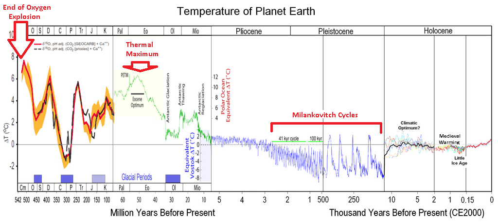
Yet the periods between glacial maxima have not stayed constant over the last 2 Ma or so (Figure showing Phanerozoic climate changes). About 0.8 to 1 Ma ago a sequence with roughly 41 ka spacing was replaced by another about every 100 ka, i.e. both overall climate periods matched one of the astronomical forcings. What is a puzzle is that the current periodicity seems to follow the very weakest influence in energy terms; that from orbital eccentricity. The energy shifts from changes in orbit shape are, in fact, far too weak to drive the accumulation and eventual melting of ice sheets on land. Climatologists have suggested a variety of processes that might be paced by eccentricity but which act to amplify is climatic ‘signal’. None have been especially convincing.

In an attempt to resolve the mystery Ayako Abe-Ouchi of the University of Tokyo and Japanese, US and Swiss colleagues linked a climate model driven by Milankovitch insolation and variations in CO2 recorded in an Antarctic ice core with a model of how land-ice forms and interacts with the underlying lithosphere (Abe-Ouchi, A. et  al. 2013. Insolation-driven 100,000-year glacial cycles and hysteresis of ice-sheet volume. Nature, v. 500, p. 190-193).

CLIMAP map of ice sheets, sea temperature chan...
Map of ice sheets, sea temperature changes, and changes in the outline of coastal regions during the last glacial maximum. (credit: Wikipedia)

Their key discovery is that the ice-sheets that repeatedly formed on the Canadian Shield and extended further south than Chicago had such a huge mass that they changed the shape of the land surface beneath them so much it had an effect on climate as a whole. The reason for this is that glacial loading forces the lithosphere down by displacing the more ductile asthenosphere sideways. But when melting begins rebound of the rock surface lags a long time behind the shrinking ice volume – well displayed today in Britain and Scandinavia by continued rise of the land to form raised beaches. In the case of the North American ice sheet, what had become an enormous ice bulge at glacial maxima developed into a huge basin up to 1 km deep as the ice began to melt. Simply by virtue of its low elevation this sub-continental basin would have warmed up more and more rapidly as the ice-surface fell because of this ‘isostatic’ lag.

Another feature to emerge from the model was the interaction between the 100 ka eccentricity ‘signal’ and that of precession at 23 ka. For long periods that kept summer temperature low enough for snow to pile up and become glacial ice, but on a roughly 100 ka time scale both acted together to increase summer temperatures at high northern latitudes. Melting that instantaneously removed some ice load each summer brought into play the sluggish isostatic  response that helped even more warming the following year. As well as convincingly accounting for the 100 ka mystery, the model explains the far more rapid deglaciations in that mode than in the preceding 41 ka cycles, which were almost symmetrical compared with the more recent slow accumulation of continental ice sheets over ~90 ka followed by almost complete melting in a mere 10 ka.

If true, the model seems to imply that before 800 ka the positions, thicknesses and extents of continental ice sheets were different from those in later times. Or perhaps it reflects a steady increase in the overall volume of ice being produced over northern North America, or that glacial erosion thinned the crust until changing isostatic influences could ‘trip’ sufficient additional warming.

Yet another risk of arsenic exposure

The most widely feared risk of poisoning through natural causes, which grossly disfigures and kills through a range of cancers, is from chronic exposure to arsenic in drinking water. Tragically, the risk is highest from what has traditionally been considered safest source, groundwater. That was the gruesome lesson of a massive transfer in Bangladesh from drinking surface water containing organic pathogens to reliance on well waters. The greatest mass poisoning in history was eventually traced to shallow aquifers in the Ganges-Brahmaputra plains that were rich in organic matter. Their reducing chemistry broke down iron hydroxide coatings on sedimentary grains. Since these minerals are among the most accommodating adsorbers of ions from the environment, including a variety of arsenic-bearing ions, their dissolution releases potential poisons from otherwise safe storage. In Bangladesh and neighbouring West Bengal in India it was found that deeper aquifers have oxidising chemistry and so the iron minerals not only hold ionic pollutants fast by adsorption but help to extract them from groundwater. Deep wells together with various kinds of treatment of shallow groundwater, some using the very iron minerals whose breakdown caused the pollution, are helping to mitigate the perilous situation for people of South Asia.

Skin lesions from arsenic poisoning in Bangladesh
Skin lesions (keratoses) from arsenic poisoning in Bangladesh (Photo credit: waterdotorg)

Much the same kind of arsenic pollution has subsequently been revealed in groundwaters of lowland Vietnam and Cambodia. Yet the turn there to deep groundwater has revealed a new twist. That too is yielding increasingly high arsenic concentrations, but for a different reason (Erband, L.E. et al. 2013. Release of arsenic to deep groundwater in the Mekong Delta, Vietnam, linked to pumping-induced land subsidence. Proceedings of the National Academy of Science, doi/10.1073/pnas.1300503110). Scientists from Stanford University, California analysed waters from around 900 wells in the Lower Mekong Delta and found several tracts with arsenic contents well above levels deemed safe by the WHO. Some, as could be anticipated from South Asian studies, were from shallow wells along the present course of the Mekong. However, in the delta area to the southwest of Ho Chi Minh City (formerly Saigon) is a large cluster from wells 150 to 450 m deep, totally unlike the situation in other areas of thick Pliocene to Recent river sedimentation.

Comparing the distribution of affected wells with precise estimates of the subsidence rates of the land surface from orbital interferometric radar surveys shows a close correlation of arsenic contamination with rates of subsidence. This suggests that groundwater pumping from deep aquifers is causing compaction at depth, in much the same way as in the environs of Venice. But is this somehow drawing in arsenic polluted water from higher levels? It seems not. So the pollution seems most likely to be an effect of pumping itself. The authors suggest that most of the subsidence is due to compaction of clay-rich sediments rather than the sandy aquifers, well known by engineers to resist compression. They explain the increasing arsenic concentrations by the introduction into the aquifers of water expelled from the clays, either containing arsenic ions in solution or carrying organic compounds that create the reducing conditions to break down iron hydroxide grain coatings and release ions adsorbed on their surfaces.

This presents another grim prospect for South Asian people forced to make the choice between drinking polluted surface water and enteric disease and increasingly exploited deep groundwaters that seem to be safe as well as in very high volumes. Let’s hope that arsenic monitoring can be maintained in the Ganges-Brahmaputra plains in the long term.

Last common paternal and maternal ancestors closer in time

One of the oddities of using human genetic material passed down the male (from Y chromosomes) and female lines (from mitochondria) to assess when fully modern humans originated is that they have hitherto given widely different dates: 50 to 115 ka and 150 to 240 ka respectively. Twice to three-times the age for a putative ancestral ‘mother’ compared with such a ‘father’ for humanity raised all kinds of problematic issues for palaeoanthropology, such as a possibly greater ‘turnover’ of lines of descent among males perhaps due to riskier lifestyles. Y-chromosome data  limited speculation on the timing of human colonisation outside of Africa to a maximum of 60 ka, even though there is fossil and archaeological evidence for a much earlier presence in the Levant and India.  The difference also questions the validity of molecular-clock approaches to evolutionary matters. Two new studies have lessened the phylogenetic  strains.

One examines Y chromosomes in 69 males from nine diverse populations from Africa, Eurasia and Central America (Poznik, G.D.  and 10 others 2013. Sequencing Y chromosomes resolves discrepancy in time to common ancestors of males versus females. Science, v. 341, p. 562-565). The US-French team applied sophisticated statistics as well as the elements of a molecular clock approach to both Y-chromosome and mitochondrial DNA, discovering in the process a hitherto unresolved feature in the African part of the male ‘tree’. The outcome is a significant revision of both male and female paths of descent: 120 to 156 ka and 99 to 148 ka to the last common ancestor in both lines. The upper limit is somewhat lower than the age of fossil evidence for the earliest anatomically modern humans.

The second study zeros-in on the European story, by examining the Y-chromosome data of 1200 men from Sardinia (Francalacci, P. and 38 others. Low-pass DNA sequencing of 1200 Sardinians reconstructs European Y-chromosome phylogeny. Science, v. 341, p. 565-569) calibrated to some extent by the date when Sardinia was first colonised (7.7 ka). It too revealed new detail that enabled the Italian-US-Spanish team to refine the time when features of Sardinian Y-chromosome DNA would coalesce with those from the rest of the world. In this case the date for a last common paternal ancestor goes back to between 180 to 200 ka, more similar to the old dates for ‘African Eve’ and the earliest modern human fossils than to either that for male or female lines arrived at by Posnik et al. (2013), which are significantly younger.

Map of early migrations of modern humans
Map of early migrations of modern humans based on Y chromsome data (credit: Wikipedia)

Equally interesting are the comments on both papers in the Perspectives section of the issue of science in which they appear (Cann, R.L. 2013. Y weigh in again on modern humans. Science, v. 341, p. 465-7).Rebecca Cann of the University of Hawaii Manoa considers the two sets of results from Y-chromosomes potentially capable of refining models for the migration times of modern humans out of Africa and their interactions with the archaic populations that they eventually displaced from Europe and central and southern Asia (Neanderthals, Denisovans and Homo erectus respectively). She believes that will include signs of earlier excursions that the generally accepted diaspora between roughly 60 and 50 ka seemingly constrained by the previous 50 to 115 ka estimate for the last common paternal ancestor. That would help explain the presence of modern humans in India at the time of the Toba eruption (71 ka).